RLHF: Reinforcement Learning from Human Feedback

1. Introduction: Why Do We Need RLHF?

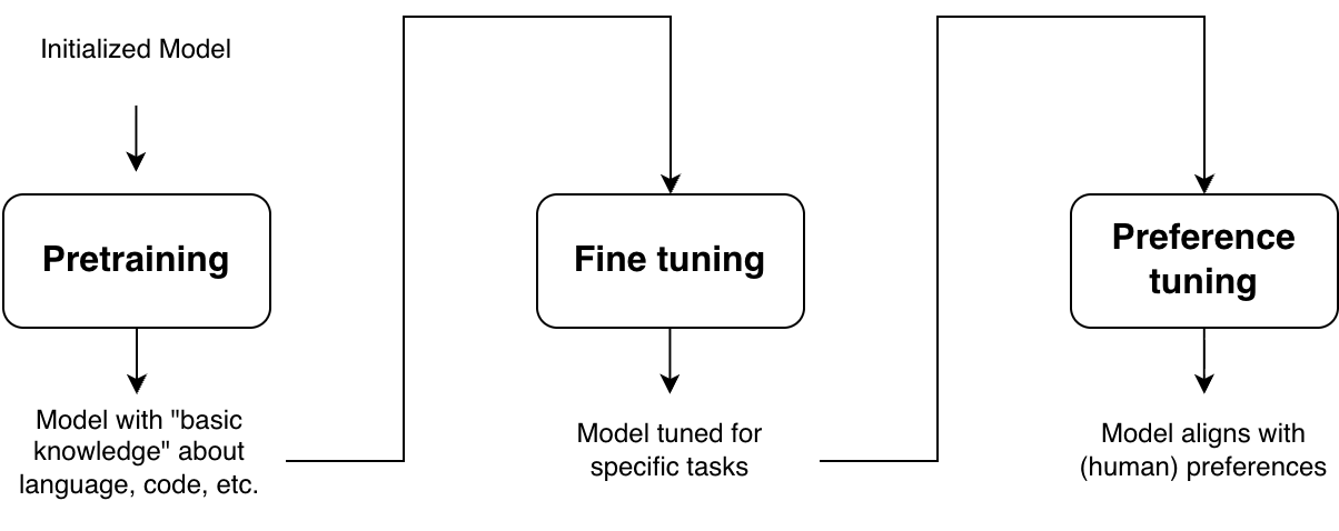
Modern AI systems, especially LLMs, are built in stages—each stage improving their capability, usefulness, and alignment with human expectations.

The journey typically begins with pretrained models. These models, such as GPT or BERT, are trained on massive amounts of text data using self-supervised objectives (e.g., next-token prediction). This stage equips the model with a broad understanding of language—grammar, facts, and general reasoning patterns. However, pretrained models are not inherently helpful or safe. They simply learn to mimic patterns in data, which may include ambiguity, bias, or undesirable behaviors.

To make these models more useful, we move to Fine-tuning/Instruction-tuning. In this stage, models are trained on curated datasets containing task-specific examples, such as question answering, summarization, or instruction-following. Fine-tuned models are significantly better at producing relevant outputs, but they still have certain limitations.

Consider the following question asked to a LLM: What’s the best way to lose weight quickly?

An instruction-tuned model is likely to generate a reasonable response such as: “Reduce carb intake, increase fiber and protein content, increase vigorous exercise.” ✔ 👍

However, the same model might also produce undesirable or harmful suggestions like: “Stop eating entirely for a few days” ❌ 👎

Instruction tuning helps the model know what to say, but it does not reliably ensure the model knows what not to say. Mathematically, instruction tuning increases the probability of preferred outputs given an input. However, it does not explicitly decrease the probability of undesirable outputs at the same time. As a result, harmful or misaligned responses may still remain in the model’s output distribution.

This gap leads to the need for alignment, ensuring that model outputs are not just statistically likely, but also aligned with what humans actually want. This is precisely where alignment methods like Reinforcement Learning from Human Feedback (RLHF)/Preference-tuning become essential, they explicitly guide the model toward human-preferred behavior while discouraging unsafe or undesirable outputs.

2. Basics of RL and How LLMs Fit In

RL is a framework where an agent learns to make decisions by interacting with an environment and receiving feedback in the form of rewards. The objective of the agent is to learn a policy that maximizes the expected cumulative reward over time.

At a high level, RL consists of:

Agent: The decision-maker (e.g., a model)
Environment: The external system the agent interacts with
State: The current context or situation
Action: A choice made by the agent
Reward: A scalar signal indicating how good the action was
Policy: A mapping from states to actions

The agent iteratively improves its behavior by trying actions, observing outcomes, and adjusting its policy to favor actions that yield higher rewards. In other term, unlike supervised learning, where the model learns from labeled examples, RL relies on trial-and-error. The agent is not explicitly told the correct action; instead, it explores different possibilities and learns from feedback.

How Do LLMs Fit into the RL Framework?

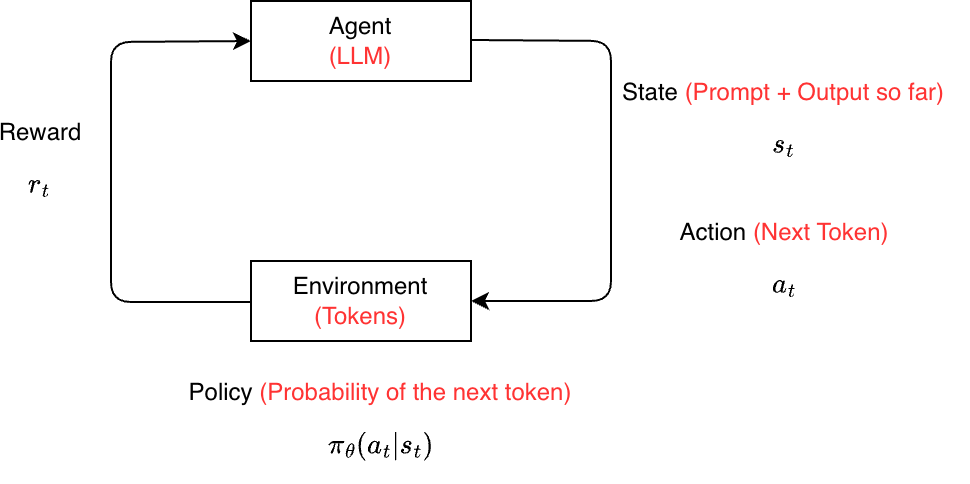
When applying RL to large language models (LLMs), we reinterpret the components of RL as follows:

RL Component	LLM Interpretation
Agent	The language model
State	The input prompt (and generated tokens so far)
Action	The next token (or sequence of tokens)
Policy	The probability distribution over tokens
Reward	A score reflecting human preference or quality

Where Does the Reward Come From?

A natural approach is to collect feedback directly from humans, for example by asking them to rate or compare model responses (e.g., thumbs up/down or ranking outputs). However, this is expensive, slow, and difficult to scale. To this end, a separate reward model is trained to approximate human preferences. This model learns from annotated comparisons and can then assign reward scores to new outputs, enabling efficient large-scale optimization without requiring continuous human involvement.

In some cases, rewards can be obtained without any human input through what are known as verifiable rewards. These are objective signals computed directly from ground truth, making them reproducible and free from human or model bias. For example, in mathematical problem solving, the reward can be based on whether the final answer exactly matches the correct solution; in code generation, whether the program passes all test cases; and in question answering, whether the predicted answer matches or overlaps with the ground truth.

3. Reward Model

A reward model takes a prompt $x$ and a generated response $y$, and outputs a scalar score $r_\theta(x, y)$ such that better responses receive higher scores than worse ones.

But who decides what is “better”?

If humans provide preferences → RLHF (Reinforcement Learning from Human Feedback)
If another LLM provides preferences → RLAIF (Reinforcement Learning from AI Feedback)
If correctness is determined by an exact verifier → RLVF (Reinforcement Learning with Verifiable Feedback)

Training the Reward Model

Architecturally, a reward model is typically a language model (encoder-only, decoder-only, or encoder-decoder). It processes the prompt-response pair, extracts representations (e.g., pre-logit embeddings), and passes them through a linear layer to produce a single scalar reward.

We assume access to binary preference data of the form: $(x, y^+, y^-)$, where $y^+$ is preferred over $y^-$. To model these preferences, we use the Bradley-Terry (BT) model, which is a statistical model for pairwise comparisons. Given items $y_i$ and $y_j$ with scores $s_i$ and $s_j$, it defines:

\[p(y_i \succ y_j) = \frac{s_i}{s_i + s_j}\]

In the LLM setting, preferences are conditioned on a prompt $x$ and we parameterize: $s(y \mid x) = \exp\big(r_\theta(x, y)\big)$. This gives:

\[p(y_i \succ y_j \mid x) = \frac{\exp(r_\theta(x, y_i))}{\exp(r_\theta(x, y_i)) + \exp(r_\theta(x, y_j))}\]

where $p$ is the probability of $y_i$ being better than $y_j$ given prompt $x$, and $r_\theta$ is the reward model.

We train the reward model by maximizing the likelihood of observed preferences:

\[\begin{aligned} \mathcal{L}(\theta) &= \mathbb{E}_{(x, y^+, y^-) \sim D} \left[\log p(y^+ \succ y^- \mid x)\right] \\ &= \mathbb{E}_{(x, y^+, y^-) \sim D} \left[ \log \frac{\exp(r_\theta(x, y^+))}{\exp(r_\theta(x, y^+)) + \exp(r_\theta(x, y^-))} \right] \\ &= \mathbb{E}_{(x, y^+, y^-) \sim D} \left[\log \sigma\big(r_\theta(x, y^+) - r_\theta(x, y^-)\big)\right] \end{aligned}\]

where $D$ is the dataset of human preferences and $y^+$ and $y^-$ are the preferred and non-preferred responses against the same input $x$. Intuitively, this objective increases the reward of preferred responses and decreases the reward of rejected ones by maximizing the difference between them.

Limitations of Reward Models

Reward models, especially those trained with pairwise (BT-style) preferences, are often biased and noisy. For instance, they may assign higher scores to longer responses even when they are less informative, simply because humans tend to prefer more detailed answers. Similarly, the presence of certain keywords or stylistic patterns can disproportionately influence the reward, regardless of actual quality. These issues arise because the model learns correlations in preference data*, not true notions of correctness or usefulness.

To address these limitations, alternative approaches move beyond binary comparisons. Instead of comparing two responses, annotators are shown a single response and asked to rate it across multiple dimensions such as: helpfulness, correctness, coherence, informativeness, etc.

This produces a vector of scores rather than a single scalar. These scores are often serialized into a string (e.g., "helpfulness: 4, correctness: 3, ...") and the model is trained to predict this string given a $(x, y)$ pair. This provides richer supervision and reduces some biases inherent in pairwise setups.

A recent paradigm is to use an LLM as a judge, where the model evaluates responses directly. This approach can be used out-of-the-box, leveraging the reasoning ability of large models. However, it comes with drawbacks such as they are less accurate than reward models trained on human preference data, often overconfident, prone to biases (e.g., verbosity bias). Nevertheless, LLM judges can also be trained explicitly. A common formulation is to model verification as a binary decision: $\log p(\text{yes/no} \mid x, y, I)$, where $I$ is an instruction such as “Is this response correct?”. The model is trained to maximize $p(\text{yes} \mid x, y^+, I)$ for correct responses, while minimize $p(\text{no} \mid x, y^-, I)$ for incorrect responses.

4. Reward Maximization Objective of LLM

We are given a reference policy $\pi_{\text{ref}}(y \mid x)$, typically an instruction-tuned LLM, and a reward model $r(x, y)$. The goal is to learn a new policy $\pi_\theta(y \mid x)$ that generates high-quality outputs according to the reward model, while still staying close to the reference policy.

Note that the reward model is imperfect as it is trained on limited and potentially biased human preference data. Optimizing only for reward can amplify these biases (e.g., favoring overly long responses) and lead to undesirable behavior. If we optimize purely for reward, the model may exploit weaknesses in the reward model, and this is known as reward hacking. The model may generate outputs that receive high reward scores but are nonsensical or unhelpful. Also, the model may collapse to a narrow set of high-reward responses, reducing diversity. To mitigate these issues, we enforce that the learned policy remains close to the reference policy.

Objective Formulation

Maximize Expected Reward: For a given prompt $x$, we want the expected reward under the policy to be high:

\[\mathbb{E}_{y \sim \pi_\theta(y \mid x)} [r(x, y)]\]

Stay Close to the Reference Policy: We measure closeness using KL divergence and we aim to minimize this divergence:

\[\mathrm{KL}\big(\pi_\theta(y \mid x) \,\|\, \pi_{\text{ref}}(y \mid x)\big) = \mathbb{E}_{y \sim \pi_\theta(y \mid x)} \left[ \log \frac{\pi_\theta(y \mid x)}{\pi_{\text{ref}}(y \mid x)} \right]\]

Final Objective (Regularized Reward): Combining both terms, we get:

\[\mathcal{L}(\theta) = \max_\theta \ \mathbb{E}_{y \sim \pi_\theta(y \mid x)} \left[ r(x, y) - \beta \log \frac{\pi_\theta(y \mid x)}{\pi_{\text{ref}}(y \mid x)} \right]\]

where $\beta$ controls the trade-off between the two loss components. This is often referred to as a KL-regularized reward objective maximization.

However, this objective involves sampling $y \sim \pi_\theta(y \mid x)$, which makes direct gradient-based optimization difficult as sampling is a non differentiable operation. Therefore, we estimate gradients of the policy.

4.1 The REINFORCE Gradient Estimator

Our goal is to estimate policy gradient:

\[\begin{aligned} \nabla_\theta\mathcal{L}(\theta) &= \nabla_\theta \mathbb{E}_{y \sim \pi_\theta(y|x)} [r(x,y)] \\ &= \nabla_\theta \sum_{y \in \mathcal{Y}} \pi_\theta(y|x) \, r(x,y) \\ &= \sum_{y \in \mathcal{Y}} \nabla_\theta \pi_\theta(y|x) \, r(x,y) \end{aligned}\]

However, this is intractable because the output space $\mathcal{Y}$ is exponentially large (all possible sequences). To address this, we aim to rewrite the gradient as an expectation. This transformation enables efficient approximation using Monte Carlo sampling, making the computation feasible in practice.

To make the gradient tractable, we apply the log-derivative trick:

\[\nabla_\theta \pi_\theta(y|x) = \pi_\theta(y|x) \nabla_\theta \log \pi_\theta(y|x)\]

Substituting this into our previous expression:

\[\begin{aligned} \nabla_\theta\mathcal{L}(\theta) &= \sum_{y} \pi_\theta(y|x) \, r(x,y) \, \nabla_\theta \log \pi_\theta(y|x) \\ &= \mathbb{E}_{y \sim \pi_\theta} \left[r(x,y) \nabla_\theta \log \pi_\theta(y|x)\right] \end{aligned}\]

This is the REINFORCE gradient estimator.

Since the expectation is still not computable exactly, we approximate it using samples. Given $N$ sample responses $y_1, \dots, y_n \sim \pi_\theta(y|x)$, we estimate:

\[\nabla_\theta \mathcal{L}(\theta) = \frac{1}{N} \sum_{i=1}^{N} r(x, y_i) \nabla_\theta \log \pi_\theta(y_i|x)\]

Although the estimator is unbiased, it often suffers from high variance, which can make training unstable. This high variance arises because:

Rewards can vary significantly across sampled outputs, especially in sequence generation tasks
The gradient depends on sampled outputs, introducing additional randomness into the updates

To mitigate this, we reduce variance by centering the rewards, i.e., subtracting the average reward (baseline) across samples:

\[\nabla_\theta \mathcal{L}(\theta) = \frac{1}{N} \sum_{i=1}^{N} \tilde{r}(x, y_i) \nabla_\theta \log \pi_\theta(y_i|x), \; \textrm{where} \; \tilde{r}(x, y_i) = r(x, y_i) - \frac{1}{N} \sum_{i=1}^{N} r(x, y_i)\]

For language models, an output sequence is given by $y = (a_1, \dots, a_T)$. The probability of the sequence factorizes autoregressively as:

\[\log \pi_\theta(y|x) = \sum_{t=1}^{T} \log \pi_\theta(a_t \mid s_t)\]

Substituting this into the REINFORCE estimator, we finally obtain:

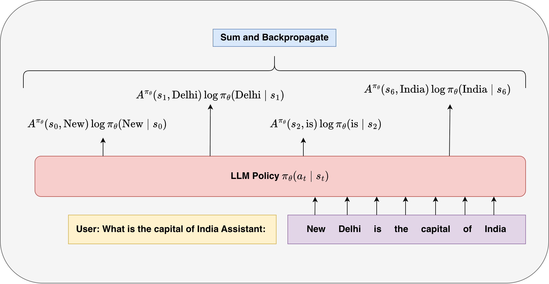
\[\bbox[15px,border:1px solid black]{ \nabla_\theta \mathcal{L}(\theta) = \frac{1}{N} \sum_{i=1}^{N} r(x,y_i) \sum_{t=1}^{T} \nabla_\theta \log \pi_\theta(a_t^i \mid s_t^i) }\]

4.2 The Credit Assignment Problem

In the above final objective, we assign the same reward to each token in the output sequence. However, this creates a fundamental challenge: Which tokens in the sequence were actually responsible for the final reward?

This is known as the credit assignment problem.

Consider a generated sentence: “The movie was absolutely terrible and I loved it.”

Suppose the task is sentiment classification and the reward is negative (correct classification).

The phrase “absolutely terrible” strongly supports the correct prediction and the phrase “I loved it” contradicts it. However, in the above formulation, both parts receive the same reward signal. This means that the helpful tokens are not specifically reinforced and the harmful tokens are not specifically penalized. This leads to inefficient and noisy learning.

4.3 Actor/Critic Method

To address credit assignment problem, we introduce the Q-function:

\[Q(s_t, a_t) = \mathbb{E}_{y_{t+1:T} \sim \pi_\theta} \left[ r(x, y) \mid s_t, a_t \right]\]

The Q-function answers the question: “If I take action $a_t$ in state $s_t$, how good is it in terms of expected future reward?”

In the context of language models:

$s_t$: the current context (previous tokens)
$a_t$: the next generated token
$Q(s_t, a_t)$: how good that token choice is, considering all possible continuations

Just as we previously reduced variance by centering the reward, we can apply the same idea at the token level by centering the Q-function. We introduce a baseline $V(s_t)$, which depends only on the state $s_t$, and define:

\[A(s_t, a_t) = Q(s_t, a_t) - V(s_t)\]

The value function itself is defined as:

\[V(s_t) = \mathbb{E}_{a_t \sim \pi_\theta} \left[ Q(s_t, a_t) \right]\]

Intuitively, the value function captures how good a state is on average. In particular, $V(s_t)$ corresponds to the expected reward obtained by continuing generation from that $s_t$ onward. It serves as a baseline expectation of future outcomes.

The advantage function $A(s_t, a_t)$ then measures how much better or worse a particular action is compared to this baseline. In other words, it tells us whether choosing token $a_t$ in state $s_t$ leads to a higher or lower reward than what is typically expected from that state. Positive advantage indicates that the action was better than average and should be reinforced, while negative advantage suggests the opposite.

Substituting this centered signal into the policy gradient yields the advantage-based formulation:

\[\nabla_\theta \mathcal(\theta) = \mathbb{E}_{y \sim \pi_\theta(y \mid x)} \left[ \sum_{t=1}^{T} A(s_t, a_t) \nabla_\theta \log \pi_\theta(a_t \mid s_t) \right]\]

In practice, the Q-function is not computed exactly. Instead, it is typically approximated using sampled rollouts from the current policy. In many sequence generation settings, we only observe a single sampled trajectory, and the Q-value is approximated using a return $R_t$. In the simplest case (e.g., sequence-level reward), this reduces to using the same final reward for all timesteps, i.e., $Q(s_t, a_t) \approx R$, where $R$ is the reward assigned to the generated sequence. More generally, $R_t$ can denote the reward-to-go from timestep $t$.

To reduce variance, we learn a value function $V_\phi(s_t)$ using a separate neural network, commonly referred to as the critic, while the policy $\pi_\theta$ is called the actor. The critic is trained to predict the expected return from a given state and typically takes as input intermediate representations of the language model (e.g., hidden states or pre-logit embeddings).

The value function is learned by minimizing the squared error between its prediction and the observed return:

\[\mathcal{L}_{\text{value}}(\phi) = \mathbb{E} \left[ \big( V_\phi(s_t) - R_t \big)^2 \right]\]

By learning this value function, we obtain a better estimate of the baseline, which reduces the variance of the policy gradient updates and leads to more stable training.

Starting from the original REINFORCE objective:

\[\nabla_\theta \mathcal{L}(\theta) = \frac{1}{N} \sum_{i=1}^{N} r(x, y_i) \sum_{t=1}^{T} \nabla_\theta \log \pi_\theta(a_t^i \mid s_t^i),\]

we improve it by introducing token-level credit assignment and variance reduction via the value function. Replacing the sequence-level reward with an advantage estimate gives:

\[\bbox[15px,border:1px solid black]{ \nabla_\theta \mathcal{L}(\theta) = \frac{1}{N} \sum_{i=1}^{N} \sum_{t=1}^{T} A(s_t^i, a_t^i)\, \nabla_\theta \log \pi_\theta(a_t^i \mid s_t^i), }\]

where the advantage is defined as:

\[A(s_t^i, a_t^i) = R_t^i - V_\phi(s_t^i).\]

5. Policy Gradient Optimization

In policy gradient methods for language models, training is inherently expensive. At every update step, we need to generate multiple trajectories (responses) autoregressively for each prompt. Since generation autoregressively itself is costly, repeating this process after every parameter update quickly becomes impractical.

To address this, we decouple data collection from optimization. Instead of generating fresh samples at every step, we first collect a large set of responses using the current policy, store them, and then reuse this data across multiple optimization steps. This reuse of trajectories significantly improves training efficiency and reduces the overall computational cost.

Importance Sampling

The key idea that enables reuse of past samples is importance sampling, which allows us to estimate expectations under one distribution using samples from another.

Consider a general expectation:

\[\begin{aligned} \mathbb{E}_{x \sim p}[f(x)] &= \sum_x p(x) f(x) \\ &= \sum_x q(x) \frac{p(x)}{q(x)} f(x) \\ &= \mathbb{E}_{x \sim q} \left[ \frac{p(x)}{q(x)} f(x) \right] \end{aligned}\]

The ratio $\frac{p(x)}{q(x)}$ is known as the importance weight, and it corrects for the mismatch between the target distribution (p) and the sampling distribution $q$. In our setting, the target distribution is the current policy and the sampling distribution is an older policy:

\[p(y) = \pi_\theta(y|x), \quad q(y) = \pi_{\theta_{\text{old}}}(y|x).\]

Using this change of measure, we can rewrite the policy gradient as an expectation over samples drawn from the old policy:

\[\bbox[15px,border:1px solid black]{ \nabla_\theta \mathcal{L}(\theta) = \mathbb{E}_{y \sim \pi_{\theta_{\text{old}}}} \left[ \sum_{t=0}^{T} r_t(\theta)\, A(s_t, a_t)\, \nabla_\theta \log \pi_\theta(a_t|s_t) \right] }\]

Here, the importance weights are defined at the token level as:

\[r_t(\theta) = \frac{\pi_\theta(a_t|s_t)}{\pi_{\theta_{\text{old}}}(a_t|s_t)}.\]

Thus, even though the data was generated using an older policy, the importance weights correct for this mismatch and allow us to obtain a valid gradient estimate for the current policy.

Optimization Procedure

Putting everything together, training proceeds in two loosely coupled phases: data collection and optimization.

Rollout Phase
- Sample a large batch of prompts
- Generate multiple outputs per prompt using $\pi_{\theta_{\text{old}}}$
Precompute Quantities
- Compute rewards
- Estimate advantages $A(s_t, a_t)$
- Store $\log \pi_{\theta_{\text{old}}}(a_t \mid s_t)$
Training Phase (Multiple Epochs)
- Shuffle and divide data into minibatches
- For each minibatch:
  - Compute $\log \pi_\theta(a_t \mid s_t)$
  - Compute importance weights $r_t(\theta)$
  - Compute objective
  - Backpropagate and update parameters
Policy Update
- Set $\pi_{\theta_{\text{old}}} \leftarrow \pi_\theta$
Repeat

The central idea is that importance sampling allows us to reuse past trajectories while still optimizing the current policy correctly. By decoupling data collection from optimization and performing multiple updates per rollout, we achieve a much more efficient training procedure, making large-scale reinforcement learning for language models practical.

6. Proximal Policy Optimization (PPO)

While importance sampling enables us to reuse past trajectories and perform multiple updates per rollout, it introduces a key challenge. If the current policy deviates too much from the behavior (old) policy, the importance weights $r_t(\theta)$ can become very large. This results in high-variance gradients and, more critically, unstable and overly aggressive updates.

However, in preference tuning, our objective is not just to improve the policy, but to do so conservatively, ensuring that the updated policy remains close to the reference (old) policy. Intuitively, we would like to increase the probability of good actions and decrease that of bad ones, but without making abrupt changes in a single update step.

PPO addresses this issue through clipping. Instead of directly using the importance weights, it constrains the update by limiting how much the ratio r_t(\theta) can influence the objective. This prevents excessively large updates and ensures that optimization remains stable.

The PPO objective is defined as:

\[L^{\text{PPO}}(\theta) = \mathbb{E}_{y \sim \pi_{\theta_{\text{old}}}} \left[ \sum_{t=0}^{T} \min\left( r_t(\theta)\, A_t,\; \text{clip}(r_t(\theta), 1 - \epsilon, 1 + \epsilon)\, A_t \right) \right]\]

where $A_t = A(s_t, a_t)$ is the advantage, and $\epsilon$ is a small constant (typically between 0.1 and 0.2) that determines the allowable deviation from the old policy.

Taking the gradient of this clipped objective yields:

\[\bbox[15px,border:1px solid black]{ \nabla_\theta \mathcal{L}^{\text{PPO}}(\theta) = \mathbb{E}_{y \sim \pi_{\theta_{\text{old}}}} \left[ \sum_{t=0}^{T} \nabla_\theta \min\left( r_t(\theta)\, A_t,\; \text{clip}(r_t(\theta), 1 - \epsilon, 1 + \epsilon)\, A_t \right) \right]. }\]

Note that the advantage $A_t$ is treated as constant with respect to $\theta$ during policy optimization (i.e., gradients do not flow through $A_t$). As a result, the gradient flows only through the importance weight $r_t(\theta)$.

The gradient flows through the active branch of the minimum. When the importance-weighted term $r_t(\theta) A_t$ lies within the clipping range, the update behaves like the standard policy gradient. However, when it moves beyond this range in a direction that would further increase the objective, the clipped term becomes active, effectively capping the update.

As a result, even if the model attempts to push the probability of an action too far, the objective no longer increases in that direction. This prevents excessively large gradients and keeps the updated policy close to $\pi_{\theta_{\text{old}}}$.

In essence, PPO strikes a balance between learning and stability: it allows the model to improve using multiple passes over the same data, while ensuring that each update remains within a controlled trust region.

7. Group Relative Policy Optimization (GRPO)

While PPO provides a stable and sample-efficient framework for training policies, it still relies on a value function to estimate advantages. In practice, this introduces additional complexity, since the critic is a separate neural network that must be trained alongside the policy. More importantly, the value function is only an approximation, and any errors in this estimation can introduce bias and instability into training. As a result, the effectiveness of PPO often depends on how accurately the critic is learned.

This naturally leads to the question: can we eliminate the critic altogether while still retaining a meaningful learning signal?

GRPO addresses this by replacing the learned value function with a relative comparison among multiple outputs for the same prompt. Instead of estimating how good an action is in absolute terms, GRPO evaluates it relative to other sampled responses. For a given prompt $x$, we sample a group of outputs $\{y_1, \dots, y_K\}$ and compute rewards for each. The advantage is then defined by normalizing these rewards within the group:

\[A(y_i) = \frac{ r(x, y_i) - \text{mean}(r(x, y_1), \dots, r(x, y_K)) }{ \text{std}(r(x, y_1), \dots, r(x, y_K)) + \epsilon }.\]

Intuitively, the notion of advantage shifts from an absolute perspective to a relative one. Instead of asking how good an action is compared to expected future rewards, we now ask how good a particular output is compared to other outputs for the same input. Outputs that perform better than the group average receive positive advantage, while those that perform worse receive negative advantage. This simple normalization removes the need for an explicit value function.

GRPO retains the same clipped PPO-style objective, but replaces token-level advantages with sequence-level relative advantages:

\[L^{\text{GRPO}}(\theta) = \mathbb{E}_{y \sim \pi_{\theta_{\text{old}}}} \left[ \sum_{t=0}^{T} \min\left( r_t(\theta)\, A(y),\; \text{clip}(r_t(\theta), 1 - \epsilon, 1 + \epsilon)\, A(y) \right) \right]\]

Note that unlike PPO, the advantage $A(y)$ is defined at the sequence level and is shared across all tokens of the sequence.

GRPO works particularly well with verifiable rewards, where correctness can be reliably determined (e.g., math problems or code execution). In such settings, the reward signal provides a consistent ranking among multiple outputs for the same prompt, which aligns naturally with GRPO’s reliance on relative comparisons within a group

8. Direct Preference Optimization (DPO)

In PPO/GRPO-style RLHF, learning proceeds in two stages. First, a reward model is learned from human preference data $(x, y^+, y^-)$:

\[\phi^* = \arg\max_{\phi} \sum_{(x,y^+,y^-)\in D} \log \sigma\big(r_{\phi}(x,y^+) - r_{\phi}(x,y^-)\big)\]

Then, the policy is optimized using this learned reward:

\[\theta^* = \arg\max_\theta \mathbb{E}_{x}\left[ \mathbb{E}_{y \sim \pi(\cdot|x)} \left[r_{\phi^*}(x,y) - \beta \, \mathrm{KL}(\pi_{\theta}(y|x)\|\pi_{\text{ref}}(y|x)) \right] \right]\]

In this formulation, human preferences $(x, y^+, y^-)$ are not used directly to optimize the policy. Instead, they are first distilled into a reward model, and the policy is trained against this learned signal under a KL constraint. While effective, this approach introduces several practical challenges: rollouts are expensive, the reward model can introduce bias due to limited preference data, and the overall pipeline becomes a complex RL optimization loop. This raises the question: can we eliminate the reward model entirely and directly optimize the policy using preference data?

DPO answers this by observing that the reward model is not fundamentally required; rather, it is a proxy for enforcing preference ordering under KL constraints. The key idea is to eliminate this intermediate step by expressing the optimal reward function $r^*$ in terms of the optimal policy $\pi^*$, and then substituting it back into the objective.

We begin with the policy optimization problem for a fixed prompt $x$:

\[\pi^* = \max_{\pi(\cdot|x)} \; \mathbb{E}_{y \sim \pi(\cdot|x)} \big[r^*(x,y) - \beta \, \mathrm{KL}(\pi(y|x)\|\pi_{\text{ref}}(y|x))\big], \; \text{subject to} \; \sum_{y} \pi(y|x) = 1\]

Expanding the expectation and KL term, and introducing a Lagrange multiplier $\lambda$ for normalization, we obtain:

\[\mathcal{L}(\pi, \lambda) = \sum_{y} \pi(y|x) r^*(x,y) - \beta \sum_{y} \pi(y|x)\log \frac{\pi(y|x)}{\pi_{\text{ref}}(y|x)} + \lambda \left(\sum_{y} \pi(y|x) - 1\right)\]

Taking the derivative with respect to $\pi(y \mid x)$ and setting it to zero yields a closed-form relation between the optimal reward and policy:

\[\frac{\partial \mathcal{L}}{\partial \pi(y|x)} = r^*(x,y) - \beta \left( \log \frac{\pi(y|x)}{\pi_{\text{ref}}(y|x)} + 1 \right) + \lambda = 0 \Longrightarrow r^*(x,y) = \beta \log \frac{\pi^*(y|x)}{\pi_{\text{ref}}(y|x)} + (\beta - \lambda)\]

This shows that the optimal reward can be written as a scaled log-ratio between the optimal policy and the reference policy.

We can also express the optimal policy as:

\[\pi^*(y|x) \propto \pi_{\text{ref}}(y|x)\exp\left(\frac{r^*(x,y)}{\beta}\right)\]

This result is crucial as it reveals that the reward model is implicitly defined by the policy itself. Building on this, we parameterize the reward model directly using the policy:

\[r_\theta(x,y) = \beta \log \frac{\pi_\theta(y|x)}{\pi_{\text{ref}}(y|x)} + \beta \log Z_x(\theta)\]

Substituting this into the original preference objective, the partition function cancels out when taking differences:

\[r_\theta(x,y^+) - r_\theta(x,y^-) = \beta \log \frac{\pi_\theta(y^+|x)}{\pi_{\text{ref}}(y^+|x)} - \beta \log \frac{\pi_\theta(y^-|x)}{\pi_{\text{ref}}(y^-|x)}\]

This leads to the final DPO objective:

\[\bbox[15px,border:1px solid black]{ \theta^* = \arg\max_\theta \sum_{(x,y^+,y^-)\in D} \log \sigma\left( \beta \left[ \log \frac{\pi_\theta(y^+|x)}{\pi_{\text{ref}}(y^+|x)} - \log \frac{\pi_\theta(y^-|x)}{\pi_{\text{ref}}(y^-|x)} \right] \right) }\]

This objective transforms the two-stage RLHF pipeline into a single-stage optimization problem that is both simpler and more stable, while still preserving the essential alignment objective.

The parameter $\beta$ in DPO originates from the KL regularization term in the RLHF objective, where it controls the trade-off between maximizing reward and staying close to the reference policy. In PPO-style training, this effect is explicit: larger $\beta$ enforces stronger penalties on deviation from the reference policy. In DPO, however, $\beta$ appears inside the sigmoid as a scaling factor.

At first glance, this suggests that increasing $\beta$ will amplify preference differences and lead to larger policy drift. However, this intuition is misleading due to the sigmoid non-linearity. If we denote the log-ratio difference as $x$, the gradient becomes:

\[\frac{\partial}{\partial x} \log \sigma(\beta x) = \beta \cdot \sigma(-\beta x)\]

As $\beta$ increases, the gradient initially grows, making the model more sensitive to preference differences. However, beyond a certain point, the sigmoid saturates, causing $\sigma(-\beta x)$ to shrink and the gradient to decrease. Thus, the learning signal does not increase monotonically with $\beta$; instead, it peaks and then diminishes.

Empirically, DPO-trained policies also tend to remain close to the reference model even without an explicit KL penalty. This is because the objective operates on the ratio $\frac{\pi_\theta}{\pi_{\text{ref}}}$, implicitly anchoring updates to the reference policy.

Therefore, $\beta$ still controls the reward–regularization trade-off, but through an implicit KL mechanism rather than an explicit penalty.

Summary

Reward Modeling: We learn a reward function from human preferences $(x, y^+, y^-)$ to capture which responses are better.
RL Objective: We formulate a KL-regularized objective to maximize reward while keeping the policy close to a reference model.
Vanilla Policy Gradient: We use REINFORCE to optimize this objective, but face high variance and instability.
Credit Assignment (Advantage): We introduce value functions and advantage estimation to assign token-level credit and reduce variance.
PPO: We stabilize training using clipping, enabling multiple updates while preventing large policy drift.
GRPO: We remove the critic by using relative rewards within a group, simplifying training.
DPO: We still rely on expensive rollouts, a biased reward model, and a complex RL pipeline. We eliminate the reward model by expressing it in terms of the policy and directly optimize using preference pairs.