Flow Matching

Generative models have rapidly evolved over the past few years, with diffusion models setting new benchmarks in image, audio, and text generation. Yet, despite their impressive performance, diffusion models often require hundreds or even thousands of sampling steps to produce a single sample.

What if we could generate high-quality samples with far fewer steps — without sacrificing performance?

This is where Flow Matching enters the picture.

In this blog, we take a closer look at the mathematical foundations of flow-based generative models, with a particular focus on Flow Matching. Flow Matching is a recent and elegant framework that learns how to continuously transport a simple probability distribution into a complex data distribution.

At its core, a flow-based model learns a transformation that maps samples from an easy-to-sample base distribution (like a Gaussian) to the data distribution. Rather than thinking of this transformation as a single jump, it is helpful to view it as a smooth trajectory: a continuous flow that gradually moves probability mass from one distribution to another.

Many popular generative approaches can be understood from this perspective. Normalizing Flows construct explicit invertible transformations. Diffusion Models define a stochastic process that gradually denoises samples toward the data distribution. Flow Matching takes a more direct route: it learns the underlying velocity field that governs this transport process.

By explicitly modeling the dynamics of how samples move through space, Flow Matching provides a principled and often more efficient way to train generative models.

Mathematical Formulation

N Let us formalize the problem:

• Let \(p_0(x)\) denote a base distribution (e.g., \(\mathcal{N}(0, I)\)) that is easy to sample from.
• Let \(p_1(x)\) denote the target distribution, i.e., the unknown data distribution.

Our goal is to transform samples \(x_0 \sim p_0\) into samples that follow \(x_1 \sim p_1\).

Instead of learning a single static mapping \(T(x)\), Flow Matching models a continuous-time transformation governed by an ordinary differential equation (ODE).

Continuous-time Flow Formulation.

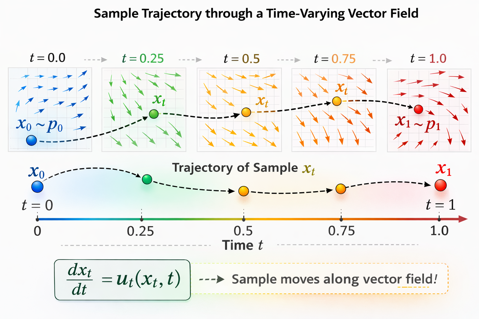
We introduce a time variable \(t \in [0,1]\), and define a trajectory \(x_t\) such that: \(x_0 \sim p_0\) and \(x_1 \sim p_1.\) We model the evolution of \(x_t\) via an ODE:

\[\frac{d x_t}{dt} = u_t(x_t),\]

where, \(u_t(x_t)\) is a time-dependent velocity field. Intuitively, the vector field \(u_t(x_t)\) tells us how a point located at \(x_t\) in space should move at time \(t\) to reach \(x_1\).

Given an initial condition \(x_0\), the ODE defines a deterministic trajectory \(x_t\) over time:

\[x_t = x_0 + \int_0^t u_s(x_s) ds\]

This ODE induces a probability flow, meaning that as samples evolve according to the velocity field, the entire distribution is transported continuously over time.

Let \(\psi_t(x_0)\) denote the solution of the ODE at time \(t\) with initial condition \(x_0\). The mapping: \(x_t = \psi_t(x_0)\) is called the flow of the ODE. The collection of trajectories \(\{\psi_t(x_0)\}_{x_0 \sim p_0}\) describes how the entire base distribution is transported to the target distribution.

Under standard regularity conditions (e.g., Lipschitz continuity), trajectories of the ODE do not intersect. Consequently, the flow is deterministic and invertible, yielding a one-to-one transformation between \(p_0\) and \(p_1\).

Evolution of Probability Density

As probability mass evolves through the vector field, the base distribution \(p_0\) is continuously transported into the target distribution \(p_1\). This transformation is described by the push-forward of \(p_0\) under the flow map \(\phi\). The transformed density at time \(t=1\) is given by the change-of-variables formula:

\[p_1(x_1) = p_0(\phi^{-1}(x_1)) \left| \det \left( \frac{\partial \phi^{-1}(x_1)}{\partial x_1} \right) \right|.\]

Equivalently, in push-forward notation: \(p_1 = \phi_* p_0\)

The evolution of the probability density \(p_t(x_t)\) is governed by the Continuity Equation. Using this, we can derive an exact equation for the log-likelihood of a sample as it transforms:

\[\frac{\partial p_t(x)}{\partial t} = - \nabla \cdot \big( p_t(x) u_t(x) \big).\]

Integrating this from \(t=0\) to \(t=1\) provides the exact log-probability of our generated data:

\[\log p_1(x_1) = \log p_0(x_0) - \int_0^1 \nabla \cdot u_t(x_t) \, dt.\]

The most intuitive training method is Maximum Likelihood Estimation. We could try to train a neural network to parameterize the vector field, \(v_\theta(x_t, t)\), and adjust the weights to minimize the negative log-likelihood loss.

\[\mathcal{L} = - \mathbb{E}_{x_1 \sim p_1} \left[ \log p_1(x_1) \right].\]

However, calculating the log-likelihood requires solving the ODE for every single training step, making the training prohibitively slow and computationally expensive.

The Flow Matching Idea

To bypass the expensive ODE solver during training, Flow Matching instead trains a neural network \(v_\theta(x_t, t)\) to directly predict the target vector field \(u_t(x_t)\) via a regression loss. The ideal Flow Matching (FM) Objective is:

\[\mathcal{L}_{FM} = \mathbb{E}_{x_t \sim p_t(x_t)} [\|v_\theta(x_t, t) - u_t(x_t)\|^2]\]

However, there is a problem that we do not know the true vector field \(u_t(x_t)\).

So how do we construct a valid target?

Conditional Flow Matching

Instead of trying to model the massive, global movement of all data at once (the marginal path), we narrow our focus to a single, specific target data point, \(x_1\). We define a conditional probability path that transports a standard Gaussian prior straight to a Dirac delta point mass localized exactly at \(x_1\). Because this path only goes to one specific data sample, its corresponding conditional vector field \(u_t(x_t \mid x_1)\) is tractable.

But how does learning the conditional vector field help us learn the marginal veector field for the entire distribution?

The marginal vector field is essentially the average of all the conditional vector fields, reweighted by how likely the target data point \(x_1\) is, given the current position \(x_t\)

Formally, we define a conditional vector field \(u_t(x_t \mid x_1)\), which is the velocity required to reach just a single known data point \(x_1\). The intractable marginal vector field can mathematically be expressed as the expectation of these conditional vector fields over the entire dataset:

\[u_t(x_t) = \int u_t(x_t \mid x_1) \frac{p_{t \mid 1}(x_t \mid x_1) q(x_1)}{p_t(x_t)} dx_1\]

where:

• \(u_t(x_t \mid x_1)\) : is a vector field which depends only on a single point \(x_1\)
• \(\frac{p_{t \mid 1}(x_t \mid x_1) q(x_1)}{p_t(x_t)}\) : is a weightage added for each \(x_1\)’s
• \(u_t(x_t)\): indicates where the particular \(x_t\) should be moved after seeing all the \(x_1\)’s

If we cannot compute the marginal vector field, can we just match the conditional one? Yes. We construct the Conditional Flow Matching (CFM) Objective:

\[\mathcal{L}_{CFM} = \mathbb{E}_{t \sim U[0,1]} \mathbb{E}_{x_1 \sim q(x_1)} \mathbb{E}_{x_t \sim p_{t|1}(x_t|x_1)} [\|v_\theta(x_t, t) - u_t(x_t|x_1)\|^2]\]

We can strictly prove that optimizing \(\mathcal{L}_{CFM}\) yields the exact same gradients for our neural network as the intractable \(\mathcal{L}_{FM}\). We start by expanding the squared \(L_2\) norm of the marginal loss \(\mathcal{L}_{FM}\):

\[\mathbb{E}_{x_t \sim p_t(x_t)} [\|v_t(x_t)\|^2 - 2 v_t(x_t) \cdot u_t(x_t) + \|u_t(x_t)\|^2]\]

We then substitute our integral definition of \(u_t(x_t)\) into the cross-term:

\[\mathbb{E}_{x_t \sim p_t} [2 v_t(x_t) \cdot u_t(x_t)] = 2 \int v_t(x_t) \cdot \left[ \int u_t(x_t|x_1) \frac{p_{t|1}(x_t|x_1) q(x_1)}{p_t(x_t)} dx_1 \right] p_t(x_t) dx_t\]

The \(p_t(x_t)\) terms conveniently cancel out, allowing us to swap the integrals:

\[\begin{aligned} &= 2 \iint v_t(x_t) \cdot u_t(x_t \mid x_1) p_{t \mid 1}(x_t \mid x_1) q(x_1) dx_1 dx_t \\ &= 2 \mathbb{E}_{x_1 \sim q(x_1), x_t \sim p_{t \mid 1}(x_t \mid x_1)} [v_t(x_t) \cdot u_t(x_t \mid x_1)] \end{aligned}\]

If we similarly expand the CFM loss \(\|v_t(x_t) - u_t(x_t \mid x_1)\|^2\), we get the exact same cross-term \(2 v_t(x_t) \cdot u_t(x_t \mid x_1)\).

Therefore, we find that the difference between the marginal objective and the conditional objective is simply a matter of constants as \(\|u_t(x_t)\|^2\) and \(\|u_t(x_t \mid x_1)\|^2\) do not depend on the neural network parameters:

\[\mathcal{L}_{FM} = \mathbb{E} [\|v_t(x_t) - u_t(x_t \mid x_1)\|^2] + \mathbb{E}[\|u_t(x_t)\|^2] - \mathbb{E}[\|u_t(x_t \mid x_1)\|^2] = \mathcal{L}_{CFM} + constant\]

Designing the Flow

Since we have complete freedom to design the conditional path from the noise \(x_0\) to the data \(x_1\), what is the easiest path to choose? A straight line.

We define our conditional probability paths as a family of normal distributions:

\[p_{t|1}(x_t|x_1) = \mathcal{N}(\mu_t(x_1), \sigma_t^2(x_1) I)\]

To ensure we start at standard noise and end at the exact data point \(x_1\), we impose the boundary constraints:

\[\mu_0(x_1) = 0, \, \sigma_0(x_1) = 1, \, \mu_1(x_1) = x_1, \, \sigma_1(x_1) = 0\]

The simplest canonical transformation mapping to satisfy these constraints uses linear scaling for both the mean and standard deviation:

\[\begin{aligned} \mu_t(x_1) &= t x_1 \\ \sigma_t(x_1) &= 1 - t \quad \end{aligned}\]

This yields our chosen Gaussian distribution:

\[p_{t \mid 1}(x_t \mid x_1) = \mathcal{N}(t x_1, (1-t)^2 I)\]

The corresponding deterministic flow map \(\psi_t(x_0)\) that generates this distribution from standard noise \(x_0 \sim \mathcal{N}(0, I)\) is:

\[\psi_t(x_0) = \sigma_t(x_1) x_0 + \mu_t(x_1)\]

Plugging in our chosen parameters gives us the canonical linear interpolation between noise and data:

\[x_t = (1-t)x_0 + t x_1\]

Deriving Target Conditional Vector Field

To train our network, we need the exact conditional vector field for this path. The general formula for a conditional vector field mapping normal distributions is:

\[u_t(x_t \mid x_1) = \frac{\sigma'_t(x_1)}{\sigma_t(x_1)} (x_t - \mu_t(x_1)) + \mu'_t(x_1)\]

For our linear path, taking the derivative with respect to time \(t\) yields:

\[u_t(x_t|x_1) = \frac{x_1 - x_t}{1 - t}\]

By substituting our definition of \(x_t\), the formula simplifies dramatically:

\[u_t(x_t|x_1) = \frac{x_1 - (t x_1 + (1-t) x_0)}{1-t} = \frac{(1-t)(x_1 - x_0)}{1-t} = x_1 - x_0\]

The Final Training Objective

The network just needs to predict the straight line from noise to data. The final Flow Matching objective is:

\[\mathcal{L} = \mathbb{E}_{t \sim U[0,1]} \mathbb{E}_{x_1 \sim p_1} \mathbb{E}_{x_0 \sim p_0} [\|v_\theta(x_t, t) - u_t(x_t \mid x_1)\|^2]\]

Which simplifies completely to:

\[\bbox[15px,border:1px solid black]{ \mathcal{L} = \mathbb{E}_{t \sim U[0,1], x_1 \sim p_1, x_0 \sim p_0} [\|v_\theta(x_t, t) - (x_1 - x_0)\|^2] }\]

Training becomes extremely simple:

1. Sample \(x_1 \sim p_1\)
2. Sample \(x_0 \sim p_0\)
3. Sample \(t \sim \mathcal{U}[0,1]\)
4. Construct \(x_t = (1 - t)x_0 + t x_1\)
5. Regress toward \(x_1 - x_0\)

No ODE solver required during training.

Inference

Once the neural network has been trained to predict the vector field, the process of generating new data is straightforward . We start from random noise \(x_0\) and numerically integrate the ODE forward in time:

\[x_1 = x_0 + \int_0^1 v_\theta(x_s, s) ds\]

In practice, we approximate this integral numerically. The simplest method is Euler integration. The Euler method discretizes the continuous time variable \(t \in [0, 1]\) into a finite number of steps to simulate the flow.

Here is the step-by-step algorithm:

1. Initialize: Sample an initial point from the base prior distribution (pure Gaussian noise), $x_0 \sim \mathcal{N}(0, I)$.

2. Define Time Steps: Choose the total number of integration steps \(T\), which defines our step size \(\Delta t = \frac{1}{T}\).

3. Iterate: For each time step \(t\), do: \(x_{t+\Delta t} = x_t + \Delta t \cdot v_\theta(x_t, t)\)

4. Output: After completing all steps, the final updated position is output as the generated data sample \(x_1\)

Flow Matching Visualization

To better understand how Flow Matching transports probability mass, the following animation shows the full transformation from the base distribution to the target distribution. As time progresses, you can see how probability mass is smoothly transported, splitting and concentrating into the four target clusters.

Although Flow Matching is often associated with straight-line transport under linear interpolation, notice that the trajectories of certain samples are not straight even in this simple example. This is because the neural network learns a global velocity field that jointly transports the entire distribution, rather than enforcing independent straight paths for each individual sample.

s