Variational AutoEncoders

Variational Autoencoders (VAEs) are a class of generative models in deep learning that go beyond simply compressing data into a latent representation. Unlike standard Autoencoders, which just learn how to encode and decode inputs, VAEs aim to learn the underlying probability distribution that generates the data itself. This probabilistic viewpoint is what makes VAEs powerful. Once the model learns the underlying data distribution, it can generate new and realistic samples, such as images, audio, or text, that closely resemble the input data that the model has never seen. In this blog post, we will delve into the mathematical formulation of VAEs and develop an understanding of how VAEs work.

1. Latent Variable Models

Before we dive into VAEs, it is helpful to understand the latent variable models (LVMs) on which they are built. These are probabilistic models that assume the data we observe is generated by some hidden structure. This hidden structure is represented by latent (or unobserved) variables. A classic example is the Hidden Markov Model (HMM), where we only observe the outputs, while the underlying states that generate them remain hidden.

Formally, suppose we have data \(\mathcal{X} = \{x_1, \dots, x_N \} \overset{\text{iid}} \sim p_x\), and we choose a parameteric family \(p_{\theta}\) to model it. The latent variable model is then defined as:

\[\begin{aligned} p_{\theta}(x) &= \sum_z p_{\theta}(x,z) \quad \text{when } z \text{ is discrete} \\ &= \int_z p_{\theta}(x,z) \,dz \quad \text{when } z \text{ is continuous} \end{aligned}\]

Intuitively, instead of modelling \(x\) directly, we can imagine that a latent variable \(z\) is sampled first and then generate an observation \(x\) conditioned on it.

Examples of LVMs:

Clustering. Here \(z \in \{1, \dots ,M \}\) is a discrete variable assigning each data sample \(x_i\) to one of \(M\) cluster, while \(x \in \mathbb{R}^d\) is the observed feature vector. The posterior \(z_i \mid x_i\) tells us which cluster best explains the point \(x_i\). Models like GMMs and K-Means fall under this category.
Feature Extraction. Here the latent space is continuous: \(z \in \mathbb{R}^k\), \(k<d\). Each latent vector \(z_i\mid x_i\) represents a low-dimensional feature vector corresponding to \(x_i\). An autoencoder model can be interpreted as an LVM model under this class.

LVMs can also be used as generative models, and we will see how VAEs build on them.

1.1 General Principle for Learning LVMs

Suppose we are given a data \(\mathcal{X} = \{x_1, \dots, x_N \} \overset{\text{iid}} \sim p_x\) and we pick a parameteric family \(p_{\theta}\) that captures the underlying data distribution. Learning a model essentially means learning the model distribution such that it closely matches with the true data distribution. This idea can be captured via KL divergence:

\[\theta^* = \arg \min _{\theta} \mathcal{D}_{KL} (p_x \| p_{\theta}) = \arg \min_{\theta} \bigg(\int_x p_x(x) \log\bigg(\frac{p_x(x)}{p_{\theta}(x)} \bigg)\, dx \bigg) = \arg \min_{\theta} \int_x-p_x(x)\cdot \log(p_{\theta}(x)) \,dx = \arg \max_{\theta} \mathbb{E}_{p_x} [\log(p_{\theta}(x))]\]

So the entire goal ends to maximum likelihood estimation.

To simplify notation, let’s focus on the loss for one training sample. Once we derive the per-sample objective, we can aggregate it over a minibatch in practice. For a single sample \(x\), the training loss becomes: \(l(\theta) = -\log(p_{\theta}(x))\)

1.2 Introducing Latent Variables

When we use an LVM, the model likelihood can be represented as the marginal of a joint distri ubution:

\[\log(p_{\theta}(x)) = \log(\int_z p_{\theta}(x,z) \,dz)\]

This integral is often a troublemaker since its intractable. Therefore, we rewrite it using an arbitrary posterior distribution \(q(z\mid x)\):

\[\log(p_{\theta}(x)) = \log \bigg(\int_z q(z\mid x) \frac{p_{\theta}(x,z)}{q(z\mid x)}\, dz \bigg) = \log \mathbb{E}_{q(z\mid x)} \bigg[\frac{p_{\theta}(x,z)}{q(z\mid x)}\bigg]\]

Now comes a classic trick: we apply the Jensen’s inequality to get a lower bound:

\[\log(p_{\theta}(x)) \geq \mathbb{E}_{q(z\mid x)} \bigg[\log \bigg(\frac{p_{\theta}(x,z)}{q(z\mid x)}\bigg)\bigg]\]

This lower bound is the famous Evidence Lower Bound (ELBO). It depends on two things:

the model parameters \(\theta\)
the auxiliary variational latent posterior \(q(z\mid x)\), which is an approximation to the true \(p_{\theta}(z\mid x)\)

Thus, the core optimization problem for LVMs becomes:

\[\boxed{ \theta^*, q^* = \arg \max_{\theta, q} = \mathbb{E}_{q(z\mid x)} \bigg[\log \bigg(\frac{p_{\theta}(x,z)}{q(z\mid x)}\bigg)\bigg] }\]

1.3 Where VAEs Enter the Story

If the conditional \(p_{\theta}(x\mid z)\) is simple enough, the optimal \(q^*(z\mid x)\) had a closed form solution, and the classic Expectation–Maximization (EM) algorithm can efficiently maximize the ELBO. This is exactly what happens in models like Gaussian Mixture Models. However, EM fails when \(p_{\theta}(x\mid z)\) becomes intractable. Therefore, we need a way to approximate \(q^*(z\mid x)\). This is where VAEs step in.

2. VAEs formulation

A VAE is built around an idea: instead of maximizing the exact log-likelihood, which is intractble, we optimize a tractable lower bound on it. This lower bound is known as the ELBO. If we further expand the ELBO, we get two terms:

\[\begin{align} \mathcal{F}_{\theta}(q) &= \mathbb{E}_{q(z\mid x)} \bigg[\log \bigg(\frac{p_{\theta}(x\mid z)\cdot p_{\theta}(z)}{q(z\mid x)}\bigg)\bigg] \\ &= \mathbb{E}_{q(z\mid x)} [\log (p_{\theta}(x\mid z))] - \mathbb{E}_{q(z\mid x)} \log \bigg( \frac {q(z\mid x)}{p_{\theta}(z)} \bigg) \\ &= \mathbb{E}_{q(z\mid x)} [\log (p_{\theta}(x\mid z))] - \mathcal{D}_{KL}(q(z\mid x)\,\|\,p_{\theta}(z)) \end{align}\]

The first term pushes the model to reconstruct the input well whereas the second pushes the posterior \(q(z\mid x)\) toward the prior. Since the true posterior is not known, we let a neural network approximate it as \(q_{\phi}(z\mid x)\). The second neural network parameterized by \(\theta\) is a decoder to model the likelihood \(p_{\theta}(x∣z)\). Together, they form the encoder–decoder pair. With this setup, training a VAE becomes the following optimization problem:

\[\boxed{ \theta^*, \phi^* = \arg \max_{\theta, \phi} \bigg[\mathbb{E}_{q_{\phi}(z\mid x)} [\log (p_{\theta}(x\mid z))] - \mathcal{D}_{KL}(q_{\phi}(z\mid x)\,\|\,p_{\theta}(z))\bigg] = \arg \max_{\theta, \phi} \mathcal{F}_{\theta}(q_{\phi}) }\]

Before diving deeper, it helps to recall that neural networks can represent probability distributions in two broad ways:

probabilistic approach: the network direclty outputs distribution parameters (e.g., means, variances, class probabilities). Classifiers are a common example as they output a categorical distribution over classes.
Deterministic approach: the network emits a sample from the learned distribution. GAN generators fall into this category, which outputs a sample \(x\), but never exposes the distribution explicitly.

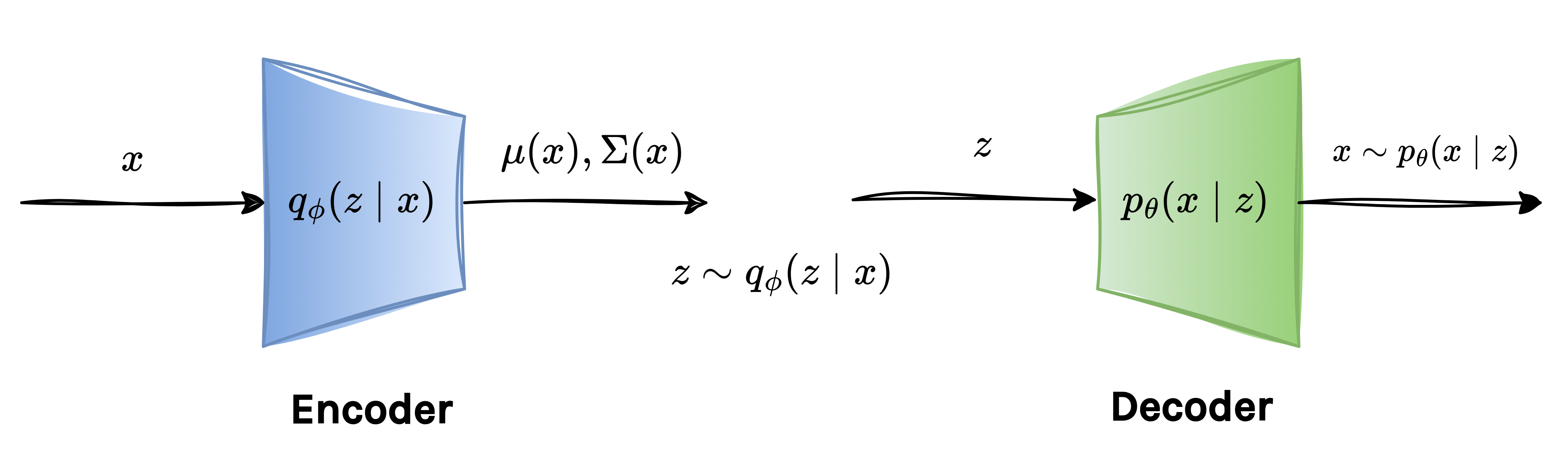
VAEs take the first approach. The encoder outputs the parameters of the approximate posterior \(q_{\phi}(z\mid x)\) and decoder outputs the parameters of the likelihood \(p_{\theta}(x\mid z)\). While the decoder is probabilistic by design, we can also view it as deterministic if we let it output the mean directly.

Below is a schematic of the VAE when the posterior \(q(x\mid z)\) is chosen to be Gaussian:

2.1 ELBO First Term

To learn the encoder parameters \(\phi\), we consider the gradient of the first term in ELBO: \(\mathbb{E}_{q_{\phi}(z\mid x)} [\log (p_{\theta}(x\mid z))]\). At first glance, this term resembles an expression of the form: \(\mathbb{E}_{p_{\phi(v)}} [f_{\phi}(v)]\). Taking the gradient of this form gives:

\[\nabla_{\phi}\, \mathbb{E}_{p_{\phi}(v)} [f_{\phi}(v)] = \nabla_{\phi} \bigg( \int_v p_{\phi}(v) \cdot f_{\phi}(v) \, dv \bigg)= \int_v \nabla_{\phi}\,(p_{\phi}(v) \cdot f_{\phi}(v)) \, dv = \int_v (\nabla_{\phi}\, f_{\phi}(v)) p_{\phi}(v) \, dv + \int_v (\nabla_{\phi}\, p_{\phi}(v))f_{\phi}(v) \, dv\]

In the above expression, the first term is an expectation and can be easily estimated using Monte Carlo samples. However, the second term is where the problem occurs as it involves \(\nabla_{\phi}\, p_{\phi}(v)\) and thus it cannot be expressed as an expectation. As a result, it cannot be computed using samples as the first term. Therefore, computing the gradient becomes intractable. We can also see it from a different view that the gradient flows through the sampling process itself. Since the sampling operation is stochastic, the gradient becomes intractable. To get around this, VAEs introduce a neat trick called Reparameterization Trick.

2.1.1 Reparameterization Trick

To bypass the non-differentiable sampling step, we rewrite the sampling step as a deterministic function of some fixed noise variable:

\[z = g_{\phi}(\epsilon), \quad \epsilon \sim p_{\epsilon}\]

Here, \(p_{\epsilon}\) is commonly a standard Gaussian and does not depend on \(\phi\). This shifts all randomness to \(\epsilon\) and makes the transformation differentiable with respect to \(\phi\). As a result, we can rewrite the expecatation as:

\[\mathbb{E}_{p_{\phi}(v)}[f_{\phi}(v)] = \mathbb{E}_{p_{\epsilon}} [f_{\phi}(g_{\phi}(\epsilon))]\]

Now the entire expression becomes differentiable with respect to \(\phi\), and backpropagation works exactly as we want. This simple reparameterization is what allows VAEs to be trained efficiently using standard gradient-based methods. The gradient of the first term in the ELBO can now be computed directly using samples:

\[\nabla_{\phi} \,\mathbb{E}_{p_{\phi}(z\mid x)}[\log(p_{\theta}(x\mid z))] = \nabla_{\phi}\, \mathbb{E}_{p_{\epsilon}(\epsilon)}[\log(p_{\theta}(x\mid g_{\phi}(\epsilon)))] = \frac{1}{M}\sum_{j=1}^{M} \nabla_{\phi} \bigg(\log(p_{\theta}(x\mid g_{\phi}(\epsilon_j))\bigg))\]

2.1.2 How to compute \(\log (p_{\theta}(x\mid z))\)?

To keep things simple, VAEs usually assume that the decoder predicts the mean of a Gaussian distribution over \(x\). Concretely,:

\[p_{\theta}(x\mid z) \sim \mathcal{N}(x; D_{\theta}(z),I),\]

where the decoder output \(\tilde{x}=D_{\theta}(z)\) acts as the mean of this Gaussian and we fix the covariance to the identity. With this assumption, evaluating the log-likelihood becomes almost trivial:

\[\log (p_{\theta}(x\mid z)) = \log \bigg(\frac{1}{(2\pi)^(d/2)} \exp(-\|x-D_{\theta}(z)\|_2^2) \bigg) \propto -\|x-D_{\theta}(z)\|_2^2\]

So, up to a constant, maximizing the log-likelihood is the same as minimizing the squared reconstruction error..

The first part of the ELBO involves taking an expectation over the encoder’s distribution \(q_{\phi}(z\mid x)\). Thanks to the reparameterization trick:

\[z_j = \mu_{\phi}(x) + \epsilon_j \cdot \Sigma_{\phi}(x),\quad j=1, \dots, M\]

we can estimate the expectation using Monte Carlo sampling:

\[\mathbb{E}_{q_{\phi}(z\mid x)}[\log(p_{\theta}(x\mid z))] = \mathbb{E}_{p_{\epsilon}(\epsilon)}[\log(p_{\theta}(x\mid g_{\phi}(\epsilon)))] \approx -\frac{1}{M}\sum_{j=1}^{M}\|x-D_{\theta}(z_j)\|_2^2,\]

In practice, we generally set the \(M=1\), so this term effectively becomes: \(\|x-D_{\theta}(z_j)\|_2^2\). This term is referred to as the reconstruction term. The objective of this term is to encourage the decoder to reconstruct the input \(x\).

Similary, we can compute easily compute its gradient with respect to the encoder parameters \(\theta\).

2.2 ELBO Second Term

So far, we have handled the first term of the ELBO. We will now similarly discuss the second term of the ELBO: \(\mathcal{D}_{KL}(q_{\phi}(z\mid x)\,\|\,p_{\theta}(z))\).

To make it easy, VAEs choose a simple prior \(p_{\theta}(z) = \mathcal{N}(0,I)\), which is independent of \(\theta\). The encoder, on the other hand, outputs a Gaussian: \(q_{\phi}(z\mid x) = \mathcal{N}(z; \mu_{\phi}(x), \Sigma_{\phi}(x))\). The KL divergence between these two Gaussians has a closed-form expression:

\[\mathcal{D}_{KL}(q_{\phi}(z\mid x)\,\|\,p_{\theta}(z)) = \mathcal{D}_{KL} (\mathcal{N}(z; \mu_{\phi}(x), \Sigma_{\phi}(x))\| \mathcal{N}(0,I)) \propto f(\mu_{\phi}(x), \Sigma_{\phi}(x))\]

where \(f\) is simply the analytic KL formula. Because of this, the gradient of the KL term with respect to encoder parameters \(\phi\) is pretty straightforward to compute.

Since the second term is independent of \(\theta\), we do not need to take its gradient with respect to the encoder parameters \(\theta\).

2.3 The Final VAE Objective

If we enforce \(q_{\phi}(z\mid x)\) to be close to \(\mathcal{N}(0,I)\) for all \(x\), then the decoder have difficulty in reconstructing. For given input samples \(x_1\) and \(x_2\), we have \(q_{\phi}(z\mid x_1) = q_{\phi}(z\mid x_2) = \mathcal{N}(0,I)\). When \(z_1 \sim q_{\phi}(z\mid x_1)\) and \(z_2 \sim q_{\phi}(z\mid x_2)\), the decoder will not be able to differentiate between \(z_1\) and \(z_2\) as they come from the same distribution and thus will result in the posterior collapse problem. Therefore, we add the weightage on the KL divergence term in ELBO. Consequently, the final VAE objective becomes:

\[\boxed{ \theta^*, \phi^* = \arg \min_{\theta, \phi} \bigg(\,\|x-D_{\theta}(z)\|_2^2 + \beta \cdot \mathcal{D}_{KL}(q_{\phi}(z\mid x)\,\|\,p_{\theta}(z))\bigg) }\]

Higher \(\beta\) may lead to posterior collapse. In contrary, lower \(\beta\) will put more emphasis on reconstruction and consequently generation quality may suffer. Therefore, both terms needs to have a balance without adversarly affecting the generation ability.

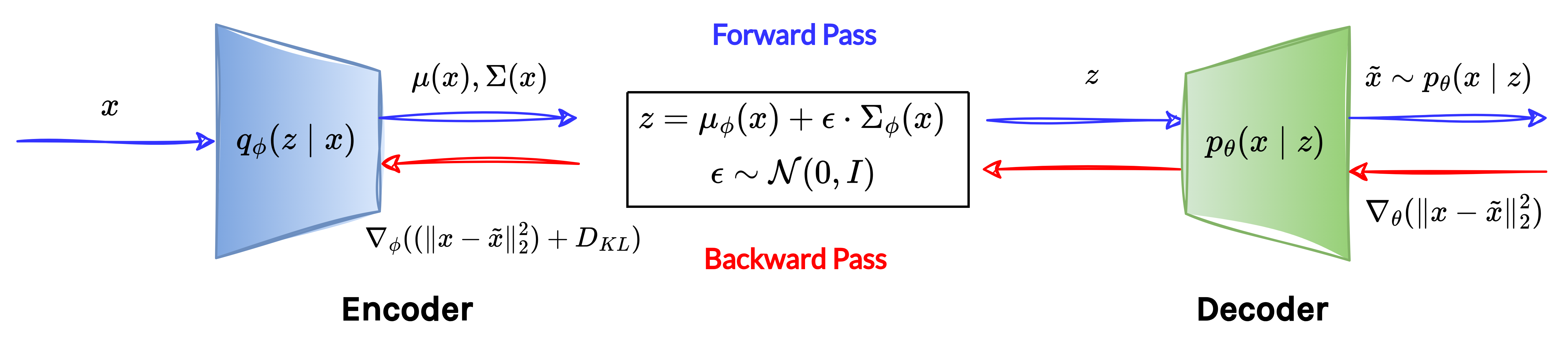
The following diagram provides an overview of the VAE training pipeline:

3. VAE Inference

VAEs are useful for two tasks once trained:

Posterior Inference: For a test input \(x_{\text{test}}\), we can find its corresponding latent representation \(z_{\text{test}}\) using the encoder as:

\[z_{\text{test}} = \mu_{\phi^*}(x_{\text{test}}) + \epsilon \cdot \Sigma_{\phi^*}(x_{\text{test}})\]

Data generation: During training, we enforce the posterior \(q_{\phi}(z\mid x)\) to be close to \(\mathcal{N}(0,I)\) via the KL divergence term. Therefore, during inference, we can simply sample \(z \sim \mathcal{N}(0,I)\) and pass it through the decoder to generate a new data sample: \(\tilde{x} = D_{\theta^*}(z)\)

Summary

VAEs replace the intractable log-likelihood with the Evidence Lower Bound (ELBO) and optimize this surrogate objective during training.
The VAE forward pass involves sampling from the latent space, which prevents gradients from flowing through the network.
VAEs introduce the Reparameterization Trick, turning stochastic sampling into a differentiable operation that enables efficient backpropagation.
Once trained, VAEs serves two key purposes: generation and feature extraction.

VQ-VAE is a well-known variant of the standard VAE that replaces the continuous latent space with a discrete one. Instead of learning a posterior distribution \(q_{z\mid x}\), it learns a finite set of discrete latent vectors: \(C=\{z_1, \dots, z_M\}\), called codewords. The encoder maps each input to the nearest codeword, and the decoder then reconstructs the input by conditioning directly on this selected codeword.