Understanding GANs

1. What does a generative model do?

At the core of generative modeling lies a simple idea: instead of merely recognizing patterns in the data, we aim to learn the underlying data distribution itself. Once this distribution is learned, we can sample from it to create entirely new data points that are statistically similar to what we have observed.

But why is this useful?

Because learning a data distribution is equivalent to learning how the data is created. We can produce realistic images that never existed, synthesize human-like speech, compose music, or even create videos without explicitly programming what those outputs should look like. Recent breakthroughs in generative modeling have brought this idea into the spotlight. Models such as DALL-E and SORA demonstrate how machines can produce visually compelling content.

2. General Principles of Generative Models

Formally, suppose we have a given dataset: \(\mathcal{X} = \{x_1, \dots, x_N\}, \quad x_i \overset{\text{i.i.d.}}{\sim} p_x\),

where \(p_x\) is the (unknown) data-generating distribution, called as the target distribution. The goal of a generative model is to estimate this distribution and sample from it.

Almost all generative modeling approaches can be understood through the following set of principles:

1. Model Selection. We assume a parameteric family on the probabilty density \(p_x\), denoted by \(p_{\theta}\). In modern deep learning, \(p_{\theta}\) is typically represented by a neural network.
2. Training Objective. We define and estimate a divergence (distance) metric between \(p_x\) and \(p_{\theta}\) that quantifies how well our model distribution matches the true data distribution.
3. Optimization. Finally, we solve an optimization problem over the parameters of \(p_{\theta}\) to minimize the divergence metric.

An overview of a typical generative modelling framework is as follows:

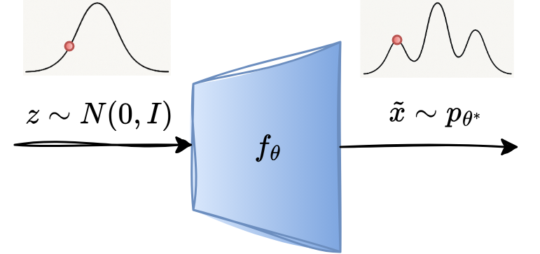
We begin with the base distribution, which is known and a simple distribution from which the sampling is easy. A common choice is an isotropic Gaussian distribution: \(Z \sim N(0,I)\).

Next, we define a mapping \(f_{\theta}: Z \rightarrow X\) that maps samples from the latent space \(Z\) to the target data space \(X\). When we pass the sample \(z\sim Z\) through \(f_{\theta}\), the output \(\tilde{x} = f_{\theta}(z)\) follows a different distribution than that of \(Z\) and is determined by the learned mapping \(f_{\theta}\). In practice, \(f_{\theta}\) is parameterized by a neural network. We denote the probability density induced by variable \(\tilde{x}\) by \(p_{\theta}\). Note that the distribution \(p_x\) is implicitly estimated by \(f_{\theta}\).

The model is trained by encouraging the generated distribution \(p_{\theta}\) to match closely with the target distribution \(p_x\). This is achieved by minimizing a divergence measure \(\mathcal{D}(.)\) between the two:

\[\theta^* = \arg \min_{\theta}\mathcal{D}\,(p_x \| p_{\theta})\]

Once the model is trained, the generation is straightforward. We draw a sample \(z\) and compute \(\tilde{x} = f_{\theta^*}(z)\). The generated sample \(\tilde{x}\) is regarded as a sample from the learned data distribution.

3. Variational Divergence Minimization

Before jumping straight into GANs, let’s take a step back and look at a more general question: How do we measure how close a model distribution is to the true data distribution using only samples? This question sits at the heart of generative modeling, and answering it will naturally lead us to the GAN framework.

Measuring Distances Between Distributions

We define a f-divergence measure between two distributions \(p_x\) and \(p_{\theta}\) as:

\[\mathcal{D}_f\,(p_x \| p_{\theta}) = \int_x p_{\theta}(x) \cdot f\bigg( \frac{p_x(x)}{p_{\theta}(x)} \bigg)\,dx,\]

where \(f:\mathbb{R}^+ \rightarrow \mathbb{R}\) is a convex, left semi continuous function and \(f(1)=0\). We observe the following properties of the f-divergence measure:

1. \(\mathcal{D}_f \geq 0\) for any choice of \(f(.)\)
2. \(\mathcal{D}_f =0\) iff \(p_x = p_{\theta}\)

For example, suppose if we choose \(f(u) = u \log(u)\), then the corresponding f-divergence becomes the KL divergence:

\[\mathcal{D}_{KL} = \int_x p_{\theta}(x) \cdot f\bigg( \frac{p_x(x)}{p_{\theta}(x)} \bigg)\,dx = \int_x p_{\theta}(x) \cdot \frac{p_x(x)}{p_{\theta}(x)} \log\bigg( \frac{p_x(x)}{p_{\theta}(x)} \bigg)\,dx = \int_x p_x(x) \cdot \log\bigg( \frac{p_x(x)}{p_{\theta}(x)} \bigg)\,dx\]

The Core Problem

Here comes the fundamental challenge:

1. Computing the f-divergence directly is intractable in high dimensional space.
2. We do not know \(p_x(x)\) and \(p_{\theta}(x)\) in closed form.
3. We only have samples.
   • samples from \(p_x\): our dataset \(\mathcal{X}\)
   • samples from \(p_{\theta}\): outputs of generator \(\tilde{x} = f_{\theta}(z)\), with \(z\sim Z\)

Spoiler Alert:

In the following explanation, our aim is to transform the divergence into an expression that looks like: \(\mathbb{E}_{p_x}[.] - \mathbb{E}_{p_{\theta}}[.]\) because expectations can be estimated directly from samples.

How do we compute \(D_f\,\)??

Trick: We use the key idea that the integrals having density functions can be approximated using the samples from the distribution via law of large numbers:

\[I = \int_x h(x) \cdot p_x(x) \,dx = \mathbb{E}_{p_x} [h(x)] = \lim_{N \to \infty} \frac{1}{N}\sum_{i=1}^{N}h(x_i), \quad x_i \overset{\text{i.i.d}} \sim p_x\]

However, in our case, \(h(x) = f\big(\frac{p_x(x)}{p_{\theta}(x)}\big)\) is not purely a function of \(x\), it depends on the unknown density ratio. So we need a clever transformation.

How do we obtain \(h(x)\,\)??

Trick: We use a concept from convex analysis.

If \(f(u)\) is convex, then there exists its convex conjugate \(f^*(t)\), defined as:

\[f^*(t) = \max_{u \in \text{domain of }f} (ut - f(u))\]

It is important to note that \(f^*(t)\) is also convex and taking the conjugate twice recovers the original function: \((f^*)^* = f\). This allows us to rewrite \(f\) itself as:

\[f(u) = \max_{t\in \text{domain of }f^*} (tu - f^*(t))\]

Now, we substitute the above expression into the definition of \(\mathcal{D}_f\):

\[\mathcal{D}_f\, (p_x \| p_{\theta}) = \int_x p_{\theta}(x) \cdot \max_{t} \bigg(t\cdot \frac{p_x(x)}{p_{\theta}(x)} - f^*(t)\bigg) \, dx\, ,\]

🧠 Now the following observation is important and allows us to finally achieve our objective. The maximization of the second term depends on the variable \(t\), while \(x\) is fixed. In other words, for every value of \(x\), we have to find the optimal \(t\) that maximizes the expression. Since the optimal \(t\) depends on \(x\), the maximizer becomes a function of \(x\) and let’s denote it by \(T^*(x)\). We can think of \(T^*(x)\) as an optimal function chosen from the space of functions \(\mathbb{T}\). With this notation, the divergence becomes:

\[\mathcal{D}_f\, (p_x \| p_{\theta}) = \int_x p_{\theta}(x) \cdot \bigg(T^*(x)\cdot \frac{p_x(x)}{p_{\theta}(x)} - f^*(T^*(x))\bigg) \, dx\,\]

As a result, we can pull out the maximization and obtain a variational lower bound on the f-divergence:

\[\mathcal{D}_f\, (p_x \| p_{\theta}) \geq max_{T(x) \in \mathbb{T}} \int_x p_{\theta}(x) \cdot \bigg(T(x)\cdot \frac{p_x(x)}{p_{\theta}(x)} - f^*(T(x))\bigg) \, dx\,\]

This expression becomes even more intuitive when written in terms of expectations:

\[\mathcal{D}_f\, (p_x \| p_{\theta}) \, \geq \, \max_{T(x) \in \mathbb{T}} \big(\mathbb{E}_{x\sim p_x}[T(x)] - \mathbb{E}_{\tilde{x} \sim p_{\theta}}[f^*(T(\tilde{x}))]\big)\]

At this stage, we have achieved an important goal: the function \(h(x)\) inside the expectations now depends on \(x\) alone.

Objective Function

We train our model to minimize the f-divergence measure:

\[\theta^* = \arg \min_{\theta}\mathcal{D}_f\,(p_x \| p_{\theta})\]

Earlier, we derived a lower bound of the f-divergence measure that depends only on expectations over samples. Therefore, optimizing this lower bound is equivalent to optimizing the original divergence. This transforms our learning problem into a minimax game:

\[\theta^* = \arg \min_{\theta} \max_{T(x) \in \mathbb{T}} \big(\mathbb{E}_{x\sim p_x}[T(x)] - \mathbb{E}_{\tilde{x} \sim p_{\theta}}[f^*(T(\tilde{x}))]\big)\]

To make this optimization practical, we parameterize \(T(x)\) using a neural network, denoted by \(T_{\omega}(x)\). This allows us to search over a large family of functions, leading to tighter lower bounds and better estimates of the divergence.

Similarly, as discussed before, we parameterize the conjugate function \(f^*\) using neural networks. Finally, the training objective becomes:

\[\boxed{ \theta^*, \omega^* = \arg \min_{\theta} \max_{\omega} \big(\mathbb{E}_{x\sim p_x}[T_{\omega}(x)] - \mathbb{E}_{\tilde{x} \sim p_{\theta}}[f^*_{\theta}(T_{\omega}(\tilde{x}))]\big) }\]

From this perspective, GAN training can be seen as a principled minimax optimization of a divergence measure. This formulation unifies many GAN variants under a common theoretical framework and also provides intuition for why GAN training naturally takes the form of a two-player game.

The objective is an adversarial optimization problem, also known as saddle-point optimization, because it involves simultaneously minimizing and maximizing the same objective function with respect to two different sets of parameters.

In practice, this is implemented using two neural networks: a generator and a discriminator. The generator is used to model \(f^*_{\theta}\) while the discriminator models \(T_{\omega}\) and we will later clarify why this network is referred to as the discriminator.

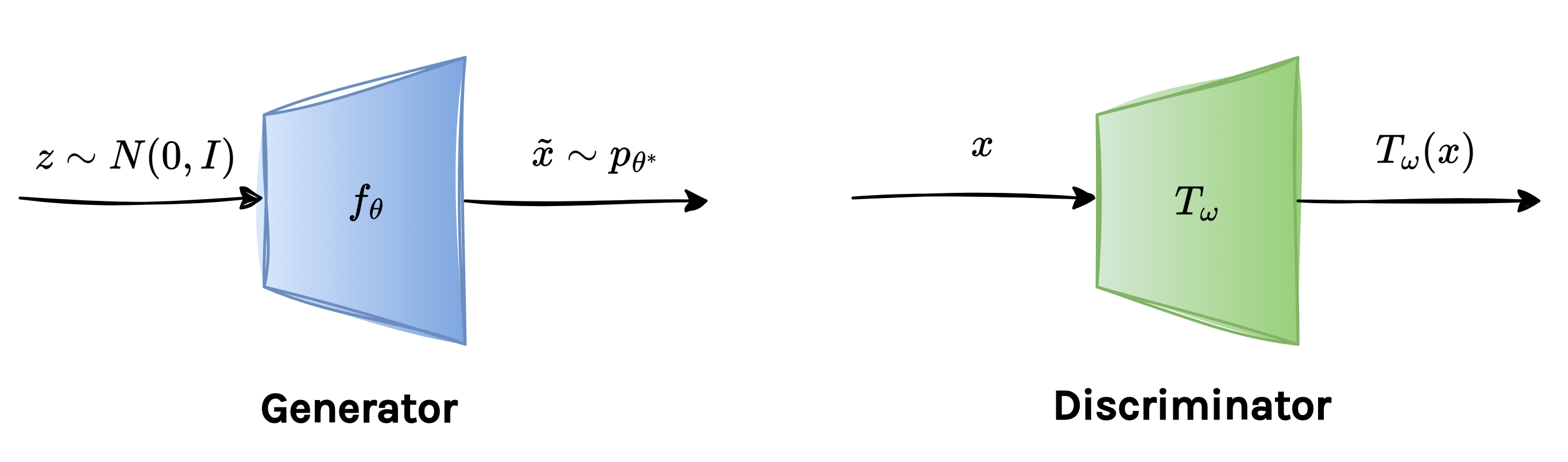
4. GANs Formulation

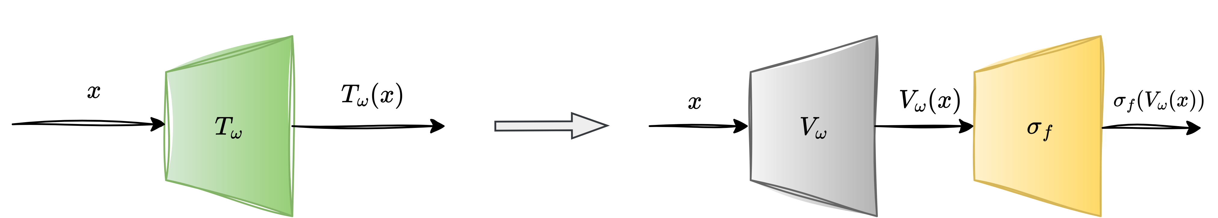
To better understand how different f-divergences fit into a unified GAN framework, it is helpful to separate what the discriminator computes from how it is constrained. We parameterize the discriminator as:

\[T_{\omega}(x) = \sigma_f(V_{\omega}(x)),\]

where \(V_{\omega}(x)\) is a neural network that outputs an unconstrained real-valued score, shared across all f-divergence variants. In other words, regardless of whether we optimize KL, reverse KL, JS, or another f-divergence, the underlying network architecture remains the same. The difference lies in the activation function \(\sigma_f\). Each f-divergence imposes constraints on the range of the variational function \(T\), which are determined by the domain of the convex conjugate \(f^*\). The role of \(\sigma_f\) is precisely to enforce these constraints, ensuring that the discriminator’s output lies in a valid range. For example, some divergences require \(T(x) \in \mathbb{R}\), while others require it to be strictly positive or bounded. With this parametrization, the variational objective takes the form:

\[J(\theta, \omega) = \mathbb{E}_{p_x}[\sigma_f(V_{\omega}(x))] - \mathbb{E}_{p_{\theta}}[f^*(\sigma_f(V_{\omega}(x)))]\]

This formulation highlights an important insight: changing the divergence does not require redesigning the discriminator network; we only adapt the activation function and its associated conjugate \(f^*\).

The original GAN formulation uses the Jensen-Shannon (JS) divergence between two distributions. The JS divergence corresponds to the following choice of the function \(f\):

\[f(u) = u\log(u) - (u+1)\log\bigg(\frac{u+1}{2}\bigg)\]

To derive a practical optimization objective, we look at the convex conjugate of \(f\), which turns out to be:

\[f^*(t) = -\log(1-\exp(t))\]

Note that the domain of \(f^*\) is \(\mathbb{R^-}\), which indicates what kind of discriminator output should be. Therefore, it allows us to choose the log sigmoid activation function for the discriminator:

\[\sigma_f(x)= -\log(1+\exp(-x)), \quad \sigma_f(.) < 0\; \forall x\]

By plugging this choice of \(f\) and its conjugate, we recover the original GAN minimax objective:

\[\boxed{ J_{\textrm{GAN}}(\theta, \omega) = \mathbb{E}_{p_x}[\log (D_{\omega}(x))] + \mathbb{E}_{p_{\theta}}[\log (1-D_{\omega}(\tilde{x}))] }\]

where the discriminator output is defined as:

\[D_{\omega}(x) = \frac{1}{1+\exp(-V_{\omega}(x))}\]

Finally, in practice, the generator and discriminator networks are implemented as:

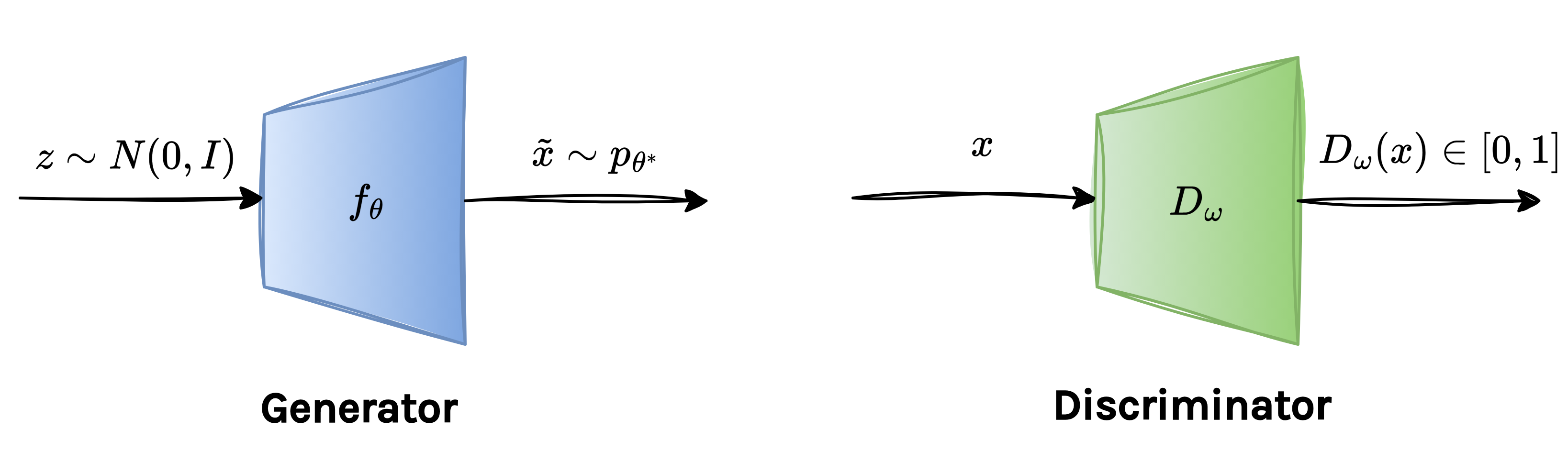
5. Implementation

Training

Training a GAN is best understood as a two-player adversarial game. The training proceeds as an alternating game, meaning that we freeze one player and let the other improve, and vice versa.

First, while optimizing the discriminator, we keep the generator parameters fixed and solve the following maximization problem:

\[\begin{aligned} \omega^* &= \arg \max \,\mathbb{E}_{p_x}[\log (D_{\omega}(x))] + \mathbb{E}_{p_{\theta}}[\log (1-D_{\omega}(\tilde{x}))] \\ &= \arg \max \, \frac{1}{B_1} \sum_{i=1}^{i=B_1} \log(D_{\omega}(x_i)) + \frac{1}{B_2} \sum_{i=1}^{i=B_2} \log(1-D_{\omega}(\tilde{x}_i)) \end{aligned}\]

Intuitively, the first term rewards the discriminator for assigning high score to real data, whereas the second term awards it for assigning low score to fake samples produced by generator. Now, this is why it explains the name discriminator: its sole task is to discriminate between real versus fake samples.

In practice, the expectations are approximated using minibatches. We use a batch of real samples: \(x_1, \dots, x_{B_1} \sim p_x\) and generated (fake) samples: \(\tilde{x}_1, \dots, \tilde{x}_{B_2} \sim p_{\theta}\)

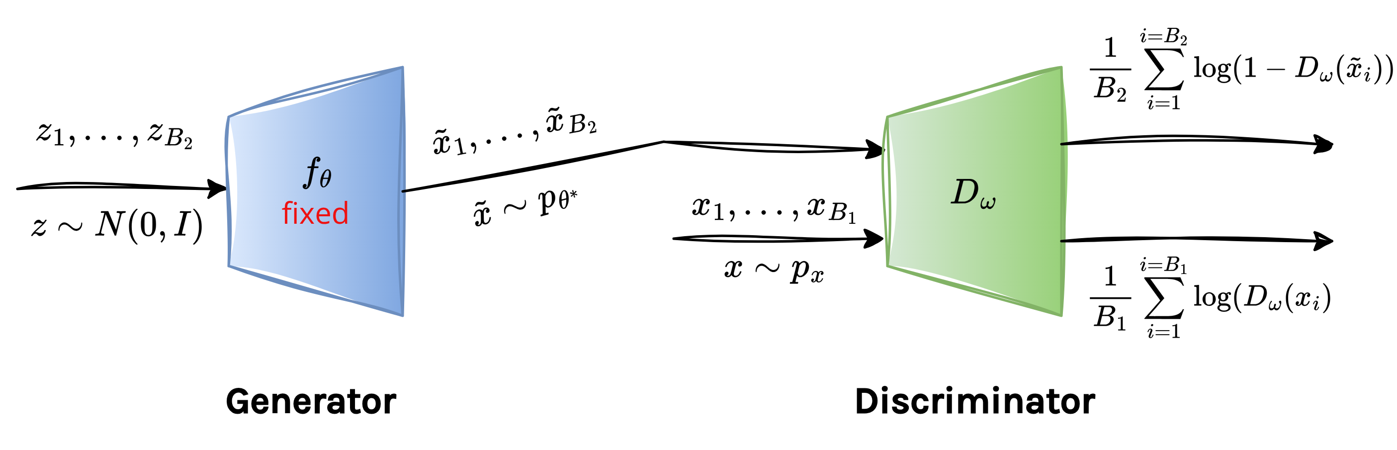
Once the discriminator has updated its parameters, we freeze it and turn to the generator. Notice that the first term in the discriminator objective depends only on real samples and therefore has no effect on the generator parameters \(\theta\). Consequently, the generator’s optimization problem simplifies to:

\[\theta^*= \arg \min \sum_{i=1}^{i=B_{2}} \log(1-D_{\omega}(\tilde{x}_i))\]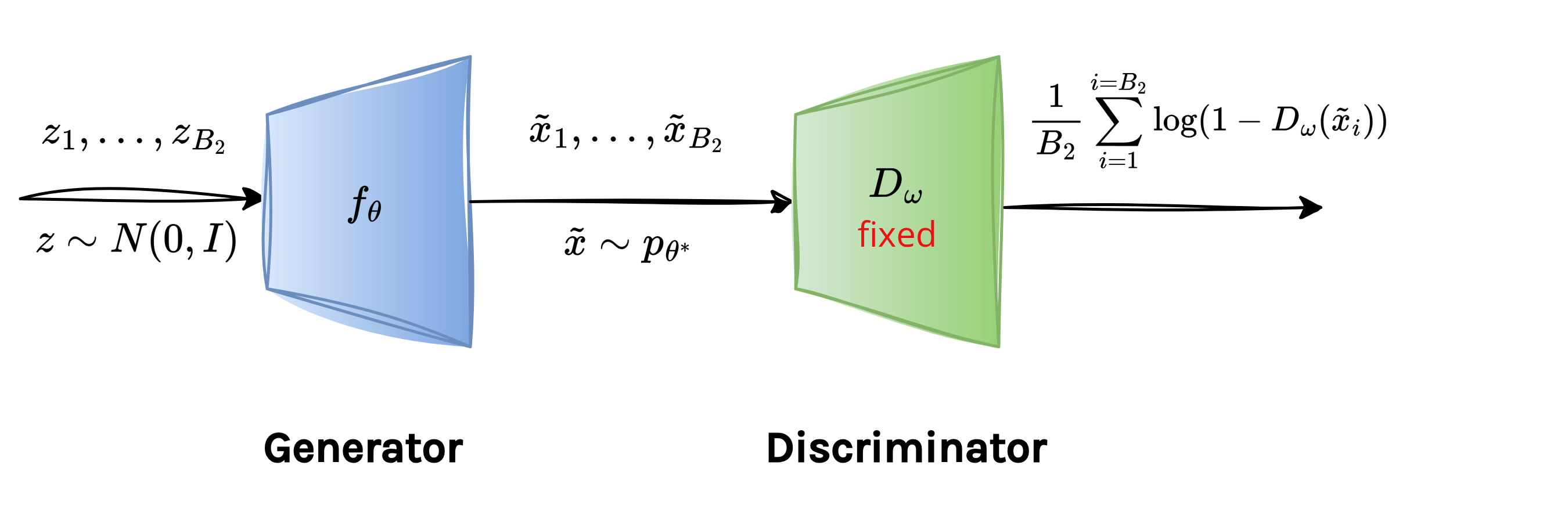

The objective indicates that the generator tries to fool the discriminator. It adjusts its parameters so that the generated samples are assigned a high score by \(D_{\omega}\).

As training progresses, this adversarial interplay ideally leads to a balance where the generator produces highly realistic samples and the discriminator becomes maximally confused.

Inference

Once the model is trained, generating new data is straightforward. We sample \(z \sim Z\) and pass it through the generator to obtain a synthetic data sample.

6. Training Instability

The key problem with f-divergence minimization is that it leads to unstable training. In high-dimensional spaces \(\mathbb{R}^d\), real-world data typically lies on a low-dimensional manifold embedded in the ambient space. In contrast, the generator initially produces samples from a different distribution whose support generally lies on another manifold. As a result, it is very likely that the supports of the real data distribution \(p_x\) and the model distribution \(p_{\theta}\) do not overlap at all. When the supports are misaligned, two problems follow:

1. Training loss saturates, and thus the generator receives near-zero gradients.
2. It can be shown that a discriminator with perfect classification accuracy always exists, which is actually not desirable.
3. Mode collapse also occurs where the generator produces samples from only a few modes of the data distribution.

7. Wasserstein GAN

To address training instability, we require a softer notion of discrepancy between distributions. This motivation leads us to the Wasserstein distance, which provides informative gradients throughout training and significantly improves stability.

The Wasserstein distance is also known as the Earth Mover’s distance or the Optimal Transport distance. It essentially measures the effort required to transform one distribution into another. Here, effort means how much probability mass is moved and how far it is moved.

What is the Wasserstein distance??

For a better understanding, we first need to understand the idea of optimal transport. Suppose \(p_x\) and \(p_{\tilde{x}}\) are two 1-D distributions. You can think of \(p_x\) as describing where the mass currently is, and \(p_{\tilde{x}}\) as describing where the mass should be. Optimal transport asks the following question: What is the most efficient way to redistribute the mass of \(p_x\) so that it exactly matches \(p_{\tilde{x}}\)?

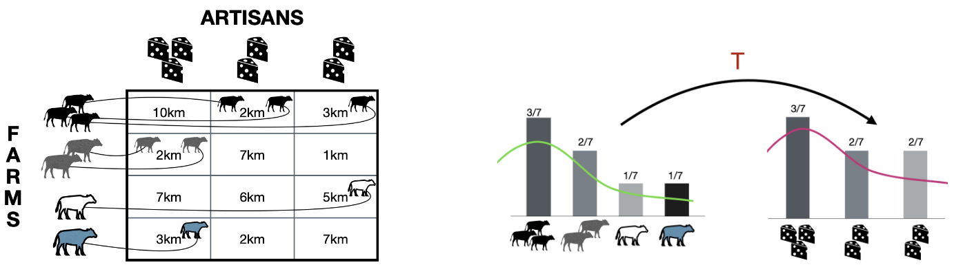
The figure above explains this concept using a cow-and-cheese-factory analogy:

• Farms have cows available at different locations along a one-dimensional axis \(x\). This represents the source distribution \(p_x\)
• Cheese factories are located at different positions and each requires a specific number of cows. This represents the target distribution \(p_{\tilde{x}}\).
• Each cell shows the distance a cow would need to travel if it were sent from a particular farm to a particular cheese factory. These distances define the cost of transportation.

An optimal transport plan specifies how many cows should be sent from each farm to each factory such that:

• All factory demands are satisfied.
• No cows are created or destroyed.
• The total transportation cost (number of cows × distance traveled) is minimized.

The curved arrows represent the transport map \(T\), which moves probability mass (cows) from the source (farms) to the target (factories). On the right side of the illustration, this idea is shown at the level of probability distributions. The bars represent how mass is distributed across locations before (\(p_x\)) and after (\(p_{\tilde{x}}\) ) transport.

How do we quantify the effort of a transport plan??

To mathematically capture this idea of effort, we introduce the following quantities:

• \(\|x-\tilde{x}\|\): the distance a unit of mass is moved.
• \(\pi(x, \tilde{x})\): the amount of mass transported from \(x\) to \(\tilde{x}\).
• \(\pi(x, \tilde{x}) \cdot \|x-\tilde{x}\|\): the work required to move that mass.

Using these, the average work (or total effort) associated with a transport plan is given by:

\[D = \int \pi(x, \tilde{x}) \cdot \|x-\tilde{x}\| \, dx\,d\tilde{x} = \mathbb{E}_{\pi(x,\tilde{x})} [\|x-\tilde{x}\|]\]

An important observation here is that a transport plan \(\pi(x, \tilde{x})\) is nothing but a joint distribution over \(x\) and \(\tilde{x}\), whose marginals correspond to \(p_x\) and \(p_{\tilde{x}}\), respectively.

Now, the question arises: Among all possible transport plans, which one requires the least amount of work?. The answer defines the Wasserstein distance.

The Wasserstein distance between two distributions \(p_x\) and \(p_{\tilde{x}}\) is defined as the minimum average transport cost over all valid transport plans:

\[W(p_x \| p_{\tilde{x}}) = \min_{\lambda \in \Pi(x, \tilde{x})} \mathbb{E}_{\lambda(x,\tilde{x})} [\|x-\tilde{x}\|],\]

where \(\Pi(x, \tilde{x})\) denotes the set of all joint distributions whose marginals are \(p_x\) and \(p_{\tilde{x}}\)

Importantly, this metric does not saturate, unlike f-divergence, when the supports of \(p_x\) and \(p_{\tilde{x}}\) do not align.

🎯 Back to GANs

In a Wasserstein GAN (WGAN), we simply replace the f-divergence objective with the Wasserstein distance:

\[\theta^* = \arg \min_{\theta} W(p_x\|p_{\theta})\]

However, computing Wasserstein distance directly is intractable in high dimensions, so we use its dual form given by:

\[W(p_x \| p_{\tilde{x}}) = \max_{\|T_{\omega}(x)\|_L < 1} \mathbb{E}_{p_x} [T_{\omega}(x)] - \mathbb{E}_{p_{\theta}} [T_{\omega}(\tilde{x})]\]

Here:

• \(T_{\omega}(x)\) is not a disciminator.
• It outputs a real-valued score.
• It has to be 1-Lipschitz.

Putting it all together, WGAN training solves:

\[\theta^*, \omega^* = \arg \min_{\theta} \max_{\|T_{\omega}(x)\|_L < 1} \mathbb{E}_{p_x} [T_{\omega}(x)] - \mathbb{E}_{p_{\theta}} [T_{\omega}(\tilde{x})]\]

To enforce the Lipschitz constraint in practice, WGAN uses weight clipping such that \(\|\omega\|_2=1\) after each gradient step.

WGANs are more stable than naive GANs because they explicitly measure how far the generator distribution is from the data distribution and not just whether they overlap.

Summary

• We first derive a generic generative modeling framework through variational f-divergence minimization.
• Using f-divergence, we arrive at the familiar minimax objective of vanilla GANs.
• Naive GANs often suffer from unstable training, especially when the supports of the model and data distributions do not overlap.
• To address this issue, we introduce Wasserstein GANs, which replace f-divergence with an optimal transport metric, leading to more stable training and meaningful gradients.

Related Topics

GANs span a wide range of ideas beyond the core formulation discussed here. From an applications perspective, important topics include GAN inversion, conditional GANs, and the use of GANs for domain adaptation. While these directions are highly relevant in practice, they fall outside the scope of this blog.