What are Diffusion Models?

Diffusion models are a family of generative models built on an idea: gradually distort the original input by adding noise, and then learn how to reverse the process. This means that starting from the original input, we repeatedly inject (diffuse) noise to it until it becomes indistinguishable from pure noise, and then we learn to denoise it iteratively until the original input is recovered. In this post, we focus on one of the most influential diffusion models, known as Denoising Diffusion Probabilistic Models (DDPMs).

If you are already familiar with VAEs, DDPMs can be viewed as a special, structured variant of VAEs, with a few key differences that are worth highlighting.

One-step vs. multi-step latent variable models

A standard VAE uses a single latent variable. Encoding and Decoding each happen in one step:
\[x \xrightarrow{\text{encoding}} z \xrightarrow{\text{decoding}} \tilde{x}\]
The latent variable \(z\) is sampled once from an approximate posterior, and the decoder attempts to reconstruct the input from it.

In contrast, diffusion models use a sequence of latent variables and operate over multiple steps. The encoding (also called the forward diffusion process) gradually adds noise, while the decoding (reverse diffusion process) removes it:
\[\begin{aligned} \text{Forward (noising):} \,& x \rightarrow z_1 \rightarrow z_2 \rightarrow \dots \rightarrow z_T \\ \text{Backward (denoising):} \,& z_T \rightarrow z_{T-1} \rightarrow z_{T-2} \rightarrow \dots \rightarrow x \end{aligned}\]
Latent space dimensionality

In VAEs, \(z\) is typically low-dimensional, whereas in DDPMs, every latent variables \(z_t\) has same dimensionality as the input \(x\).
Learned vs. fixed encoding process

In VAEs, the encoder distribution \(q_{\phi}(z\mid x)\) is learned via ELBO maximization along with the decoder. However, in DDPMs, the forward process \(q(z_t\mid z_{t-1})\) is fixed and known. It is defined as a simple Markov chain that adds Gaussian noise at each step. Only the reverse process \(p_{\theta}(z_{t-1}\mid z_t)\) is learned via ELBO maximization.

1. Mathematical Formulation

Let \(x_0 \sim p_X\) denote a data sample (e.g. an image). We introduce a sequence of latent variables \(x_1, \dots, x_T\), where \(T\) is the total number of diffusion steps. These latent variables are obtained through a forward (noising) process, which progressively corrupts the data with Gaussian noise.

1.1 Forward (Noising) Process

The forward process is defined as a first-order Markov chain:

\[x_t = \sqrt{\alpha_t}\cdot x_{t-1} + \sqrt{1-\alpha_t}\cdot \epsilon_t, \quad \epsilon_t \sim \mathcal{N}(0,I), \quad t=1, \dots, T,\]

where \(\alpha_t \in (0,1)\) is a fixed variance schedule.

Equivalently, the transition distribution is:

\[q(x_t\mid x_{t-1}) = \mathcal{N}(x_t; \sqrt{\alpha_t}x_{t-1}, (1-\alpha_t)I)\]

Unlike VAEs, where the encoder is learned, the forward process in DDPMs is fixed. By repeatedly adding Gaussian noise, the data distribution is guaranteed to converge to a standard normal distribution: \(x_T \sim \mathcal{N}(0,I)\). This eliminates the need to learn an encoder altogether.

1.2 Reverse (Denoising) Process

The goal of diffusion models is to learn how to reverse the noising process. We assume a parameterized Gaussian family for the reverse transitions:

\[p_{\theta}(x_{t-1}\mid x_t) = \mathcal{N}(x_{t-1}; \mu_{\theta}, \Sigma_{\theta}),\]

where \(\mu_{\theta}\) and \(\Sigma_{\theta}\) are implicitly learned via ELBO optimization. Intuitively, this model learns how to denoise \(x_t\) step by step, eventually recovering a clean sample \(x_0\).

2. ELBO Optimization for DDPMs

To derive the training objective, it is useful to recall the ELBO used in VAEs:

\[F_{\theta}(q_\phi) = \mathbb{E}_{q_{\phi}(z\mid x)} \log \bigg( \frac{p_{\theta}(x,z)}{q(z\mid x)}\bigg)\]

In DDMPs, the latent variables are the entire trajectory \(x_{1:T}\) and the posterior \(q(x_{1:T}\mid x_0)\) is fixed. The ELBO becomes:

\[F_{\theta}(q) = \mathbb{E}_{q(x_{1:T}\mid x_0)}\bigg[ \log \bigg( \frac{p_{\theta}(x_{0:T})}{q(x_{1:T}\mid x_0)}\bigg) \bigg],\]

Since:

\(x_T \sim \mathcal{N}(0,I)\) is fixed and independent of \(\theta\),
both the forward and reverse processes are first-order Markov,

we can factorize the joint distributions and rewrite the ELBO as:

\[F_{\theta}(q) = \mathbb{E}_{q(x_{1:T}\mid x_0)} \Bigg[ \log \Bigg(\frac{p(x_T) \, \prod\limits_{t=1}^{T} p_{\theta}(x_{t-1}\mid x_{t})}{\prod\limits_{t=1}^{T}q(x_t\mid x_{t-1})}\Bigg) \Bigg]\]

To keep the derivation readable, let us temporarily focus on the quantity inside the expectation and denote it by \(A\). Starting from the joint model and the variational posterior, we can write:

\[\begin{align} A &= \log \Bigg(\frac{p(x_T) \, \prod\limits_{t=1}^{T} p_{\theta}(x_{t-1}\mid x_{t})}{\prod\limits_{t=1}^{T}q(x_t\mid x_{t-1})}\Bigg) \\ &= \log \Bigg(\frac{p(x_T)\cdot p_{\theta}(x_0\mid x_1) \, \prod\limits_{t=2}^{T} p_{\theta}(x_{t-1}\mid x_{t})}{q(x_1 \mid x_0)\prod\limits_{t=2}^{T}q(x_t\mid x_{t-1})}\Bigg) \\ &= \log \Bigg(\frac{p(x_T)\cdot p_{\theta}(x_0\mid x_1)}{q(x_1 \mid x_0)}\Bigg) + \log \Bigg( \frac{\prod\limits_{t=2}^{T} p_{\theta}(x_{t-1}\mid x_{t})}{\prod\limits_{t=2}^{T}q(x_t\mid x_{t-1})} \Bigg) \end{align}\]

Now, lets consider the denominator in the second term. Recall that the forward (encoding) process is a Markov chain. This allows us to insert \(x_0\) without changing the conditional distribution:

\[q(x_t \mid x_{t-1}) = q(x_t \mid x_{t-1}, x_0)\]

Using Bayes’ rule, we can rewrite this as:

\[q(x_t \mid x_{t-1}) = q(x_t \mid x_{t-1}, x_0) = \frac{q(x_{t-1} \mid x_{t}, x_0) q(x_t\mid x_0)}{q(x_{t-1}\mid x_0)}\]

Substituting this expression back into \(A\), we obtain

\[\begin{align} A &= \log \Bigg(\frac{p(x_T)\cdot p_{\theta}(x_0\mid x_1)}{q(x_1 \mid x_0)}\Bigg) + \log \Bigg( \frac{\prod\limits_{t=2}^{T} p_{\theta}(x_{t-1}\mid x_{t})\color{red}{q(x_{t-1}\mid x_0)}}{\prod\limits_{t=2}^{T}\color{red}{q(x_{t-1} \mid x_{t}, x_0) q(x_t\mid x_0)}} \Bigg) \\ &= \log \Bigg(\frac{p(x_T)\cdot p_{\theta}(x_0\mid x_1)}{q(x_1 \mid x_0)}\Bigg) + \log\Bigg(\frac{q(x_1 \mid x_0)}{q(x_T \mid x_0)} \Bigg) + \log\Bigg( \frac{\prod\limits_{t=2}^{T} p_{\theta}(x_{t-1}\mid x_{t})}{\prod\limits_{t=2}^{T}q(x_{t-1} \mid x_{t}, x_0)} \Bigg) \\ &= \log \bigg(p_{\theta}(x_0\mid x_1) \bigg) + \log \bigg(\frac{p(x_T)}{q(x_T \mid x_0)} \bigg) + \log\Bigg( \frac{\prod\limits_{t=2}^{T} p_{\theta}(x_{t-1}\mid x_{t})}{\prod\limits_{t=2}^{T}q(x_{t-1} \mid x_{t}, x_0)} \Bigg) \end{align}\]

We now reintroduce the expectation with respect to the forward process \(q(x_{1:T}\mid x_0)\) and define the ELBO:

\[F_{\theta}(q) = \mathbb{E}_{q(x_{1:T}\mid x_0)} \Bigg[\log \bigg(p_{\theta}(x_0\mid x_1) \bigg) + \log \bigg(\frac{p(x_T)}{q(x_T \mid x_0)} \bigg) + \log\Bigg( \frac{\prod\limits_{t=2}^{T} p_{\theta}(x_{t-1}\mid x_{t})}{\prod\limits_{t=2}^{T}q(x_{t-1} \mid x_{t}, x_0)} \Bigg) \Bigg]\]

This expression can be further decomposed into a sum of expectations, each involving only the variables it depends on:

\[F_{\theta}(q) = \mathbb{E}_{\color{red}{q(x_1\mid x_0)}} \Bigg[\log \bigg(p_{\theta}(x_0\mid x_1) \bigg) \Bigg] + \mathbb{E}_{\color{red}{q(x_T\mid x_0)}} \Bigg[\log \bigg(\frac{p(x_T)}{q(x_T \mid x_0)} \bigg) \Bigg] + \sum_{t=2}^{T}\mathbb{E}_{\color{red}{q(x_t, x_{t-1}\mid x_0)}} \Bigg[\log\Bigg(\frac{p_{\theta}(x_{t-1}\mid x_{t})}{q(x_{t-1} \mid x_{t}, x_0)} \Bigg)\Bigg]\]

The distributions over which expectations are taken are highlighted in red. Each term depends only on the variables appearing inside it. We will now use the following property of the conditional expection for the last term:

\[\mathbb{E}_{q(x_t, x_{t-1}\mid x_0)}[.] = \mathbb{E}_{q(x_t \mid x_0)} \cdot \mathbb{E}_{q(x_{t-1} \mid x_t , x_0)} [.]\]

Applying this, the ELBO simplifies to:

\[F_{\theta} = \underbrace{\mathbb{E}_{q(x_1\mid x_0)} \bigg[\log \bigg(p_{\theta}(x_0\mid x_1) \bigg) \bigg]}_{\text{reconstruction term}} - \underbrace{\mathcal{D}_{KL} (q(x_T\mid x_0)\|p(x_T))}_{\text{prior matching term}} - \underbrace{\sum_{t=2}^{T}\mathbb{E}_{q(x_t\mid x_0)} \mathcal{D}_{KL}(\underbrace{q(x_{t-1} \mid x_{t}, x_0)}_{\color{red}{\text{known denoising}}}\|\underbrace{p_{\theta}(x_{t-1}\mid x_{t})}_{\color{red}{\text{learnable denoising}}})}_{\text{consistency term}}\]

The prior-matching term is independent of \(\theta\), so we can exclude it from the objective. In practice, the reconstruction term is often omitted. As a result, the practical DDPM objective becomes:

\[\boxed{ F_{\theta} = -\sum_{t=2}^{T}\mathbb{E}_{q(x_t\mid x_0)} \mathcal{D}_{KL}(q(x_{t-1} \mid x_{t}, x_0)\|p_{\theta}(x_{t-1}\mid x_{t})) }\]

2.1 An Intuitive Analogy

One way to build intuition for this objective is through a simple analogy—at least, this is how I like to think about it. Imagine a parent training a child to travel between home (\(x_0\)) and school (\(x_T\)). The route has total \(T\) landmarks. During training, the parent repeatedly teaches the child how to return home from school, step by step, moving from one landmark to the previous one. When all these local steps are learned well, the child eventually learns the entire route. Once the training is complete, starting from school, the child can confidently navigate back home on their own by retracing the steps one landmark at a time.

Now imagine that every parent trains their child in the same way. If you randomly pick a child and simply follow them from school, they will eventually lead you to their home.

In the same spirit, in a diffusion model, we start from a random noise sample and repeatedly apply the learned reverse steps. If each step is learned well, the process naturally guides us back to a clean data sample.

How to compute the consistency term??

To understand the DDPM training objective, we first need to derive the reverse-time posterior \(q(x_{t-1} \mid x_{t}, x_0)\) that appears inside the consistency term.

Step 1: Start from Bayes’ rule

Using Bayes’ rule, we can write:

\[q(x_{t-1} \mid x_{t}, x_0) = \frac{q(x_t \mid x_{t-1}, x_0)q(x_{t-1} \mid x_0)}{q(x_t \mid x_0)}\]

Step 2: The forward diffusion process

We know that the forward process adds Gaussian noise step by step:

\[x_t = \sqrt{\alpha_t}\cdot x_{t-1} + \sqrt{1-\alpha_t}\cdot \epsilon_t, \quad \epsilon_t \sim \mathcal{N}(0,I),\]

By recursively applying this update, we can express any noisy sample \(x_t\) directly in terms of the original data \(x_0\):

\[\boxed{ x_t = \sqrt{\tilde{\alpha}_t}x_0 + (1-\tilde{\alpha}_t)\epsilon, \quad \epsilon \sim \mathcal{N}(0,I), }\]

where \(\tilde{\alpha}_t = \prod\limits_{i=1}^{t}\alpha_i\). This gives us the marginal distribution:

\[q(x_t \mid x_0) = \mathcal{N}(x_t; \sqrt{\tilde{\alpha}_t}x_0, (1-\tilde{\alpha}_t)I),\]

We can conclude from here that the latent \(x_t\) in the forward process can be directly obtained in a single step without adding noise \(t\) times.

Step 3: The reverse posterior

Plugging the Gaussian expressions into Bayes’ rule yields:

\[q(x_{t-1} \mid x_{t}, x_0) = \frac{\mathcal{N}(x_t; \sqrt{\alpha_t}x_{t-1}, (1-\alpha_t)I)\cdot \mathcal{N}(x_{t-1}; \sqrt{\tilde{\alpha}_{t-1}}x_0, (1-\tilde{\alpha}_{t-1})I)}{\mathcal{N}(x_t; \sqrt{\tilde{\alpha}_t}x_0, (1-\tilde{\alpha}_t)I)} \\\]

As a result, the reverse process is also Gaussian, just like the forward process, but with different distribution parameters:

\[\boxed{ \begin{aligned} q(x_{t-1} \mid x_{t}, x_0) &= \mathcal{N}(x_{t-1}; \mu_q(x_t, x_0), \Sigma_{q}(t)) \\ \mu_q(x_t, x_0) &= \frac{\sqrt{\alpha_t}(1-\tilde{\alpha}_{t-1})x_t + \sqrt{\tilde{x}_{t-1}}(1-\alpha_t)x_0}{1-\tilde{\alpha}_t} \\ \Sigma_{q}(t) &= \frac{(1-\alpha_t)(1-\tilde{a}_{t-1})}{(1-\tilde{a}_{t})} I \end{aligned} }\]

Step 4: Parameterizing the reverse process

In DDPMs, we approximate the true reverse posterior with a learned Gaussian:

\[p_{\theta}(x_{t-1}\mid x_t) = \mathcal{N}(x_{t-1}; \mu_{\theta}, \Sigma_q(t))\]

Here, we only keep the mean \(\mu_{\theta}\) as a learnable parameter whereas the covariance is chosen to be a constant.

Step 5: The consistency term

The ELBO contains the KL divergence between two Gaussians distribution with the same covariance. As a result KL divergence reduces to:

\[\begin{aligned} \mathcal{D}_{KL}(q(x_{t-1} \mid x_{t}, x_0)\|p_{\theta}(x_{t-1}\mid x_{t})) &= \mathcal{D}_{KL}(\mathcal{N}(x_{t-1}; \mu_q(x_t, x_0), \Sigma_{q}(t)) \| \mathcal{N}(x_{t-1}; \mu_{\theta}, \Sigma_q(t))) \\ &\propto || \mu_q(x_t, x_0) - \mu_{\theta}||_2^2 \end{aligned}\]

Finally, the ELBO objective becomes:

\[F_{\theta} = -\sum_{t=2}^{T} || \mu_q(x_t, x_0) - \mu_{\theta}||_2^2\]

Step 6: Reparameterizing in terms of noise

Recall that,

\[x_t = \sqrt{\tilde{\alpha}_t}x_0 + (1-\tilde{\alpha}_t)\epsilon, \implies x_0 = \frac{x_t- (1-\tilde{\alpha}_t)\epsilon}{\sqrt{\tilde{\alpha}_t}}\]

Substituting \(x_0\) in \(\mu_q(x_t, x_0)\), we obtain:

\[\mu_q = \frac{1}{\sqrt{\alpha_t}}x_t - \frac{1-\alpha_t}{\sqrt{1-\tilde{\alpha}_t}\sqrt{\alpha_t}}\epsilon\]

Similarly, we reparameterize the learned mean as:

\[\mu_{\theta} = \frac{1}{\sqrt{\alpha_t}}x_t - \frac{1-\alpha_t}{\sqrt{1-\tilde{\alpha}_t}\sqrt{\alpha_t}}\epsilon_{\theta}\]

Step 7: The final training objective

Based on the derived expressions for \(\mu_q\) and \(\mu_{\theta}\), we can express the KL-divergences as:

\[\begin{aligned} \mathcal{D}_{KL} &\propto || \mu_q(x_t, x_0) - \mu_{\theta}||_2^2 \\ &\propto || \epsilon - \epsilon_{\theta}(x_t, t)||_2^2 \end{aligned}\]

Finally, the ELBO employed during training simplifies to a noise-prediction objective, where the model minimizes the regression error between the true injected noise \(\epsilon\) and its estimate at each timestep \(t\):

\[\boxed{ \theta^* = \arg \min_{\theta} \sum_{t=2}^{T} || \epsilon - \epsilon_{\theta}(x_t, t)||_2^2 }\]

3. Implementation

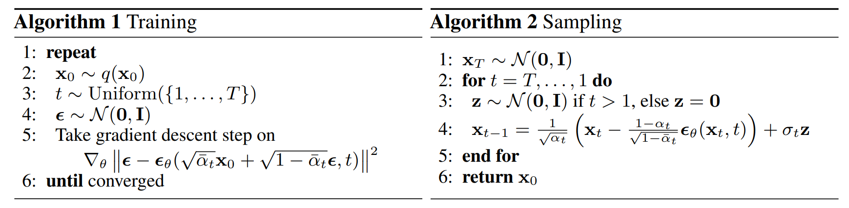
The ELBO objective involves a sum over all diffusion steps. However, computing this full sum at every training iteration would be unnecessarily expensive. Therefore, in practice, we compute only for a single time step \(t \sim \mathcal{U}\{2, \dots, T\}\), which provides an unbiased Monte-Carlo estimate of the full objective. The overall training and sampling procedures are summarized in the figure below.

Summary

DDPMs are latent variable models trained via ELBO optimization. Unlike VAEs, DDPMs employ a sequence of latent variables with a fixed, non-learnable forward (encoding) process that gradually adds noise.
The ELBO objective reduces to a simple regression objective in practice: learning to predict the injected Gaussian noise at each diffusion step.
Sample generation follows an iterative reverse-diffusion process, starting from pure noise and progressively denoising the sample. Therefore, generation is inherently sequential and relatively slow compared to one-shot generative models.

While not covered in this post, several closely related topics are worth exploring, as they play a crucial role in practical diffusion model implementations. These include commonly used neural architectures such as U-Net and Diffusion Transformers (DiT), which serve as the backbone networks for most diffusion models. Also, Denoising Diffusion Implicit Models (DDIMs) extend DDPMs by enabling inversion, and faster generation.